源码阅读及理论详解《 Informer: Beyond Efficient Transformer for Long Sequence Time-Series Forecasting 》

• Informer论文：https://arxiv.org/pdf/2012.07436.pdf
• Informer源码：GitHub – zhouhaoyi/Informer2020: The GitHub repository for the paper “Informer” accepted by AAAI 2021.
• Transformer笔记：《Attention Is All You Need》_郑烯烃快去学习的博客-CSDN博客

目录

0x01 Transformer存在的问题

0x02 Informer研究背景

0x03 Informer整体架构

（一）ProbSparse Self-attention

（二）Self-attention Distilling

（三）Generative Style Decoder

0x04 计算损失与迭代优化

0x05 源码阅读——站在巨人的肩膀上

（一）环境的搭建

（二）Informer文件框架

（三）数据的输入

（四）模型训练

（1）预处理

（2）encoder

（3）dropout

（4）Convlayer

（5）decoder

0x01 Transformer存在的问题

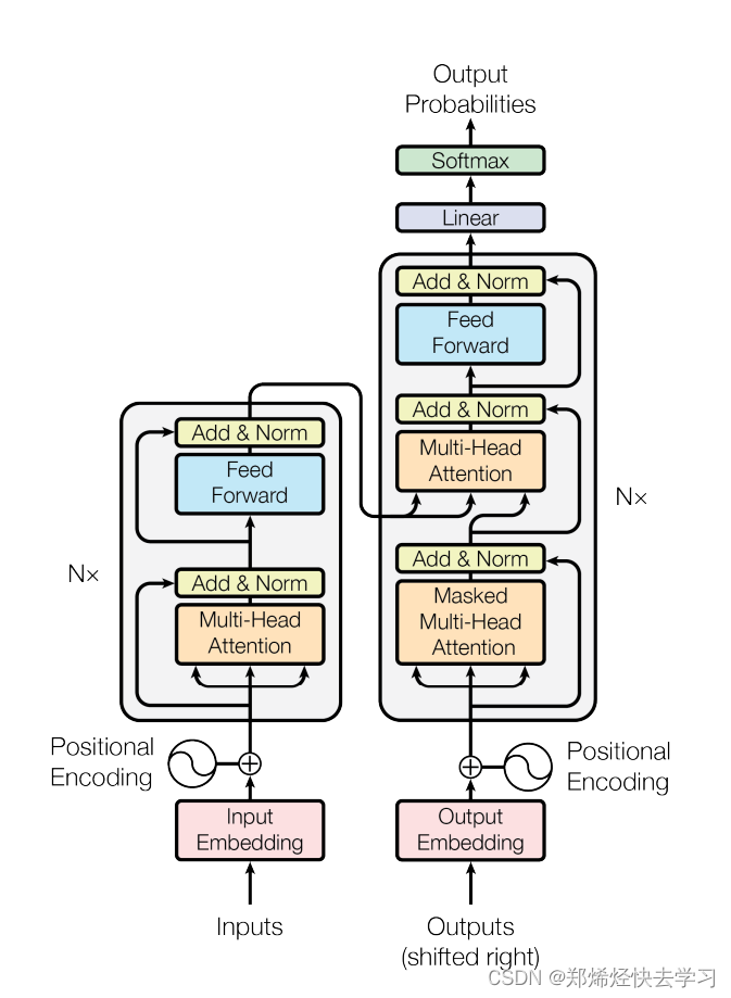
Informer实质是在Transformer的基础上进行改进，通过修改transformer的结构，提高transformer的速度。那么Transformer有什么样的缺点：

（1） self-attention的平方复杂度。self-attention的时间和空间复杂度是O(L^2)，L为序列长度。

（2） 对长输入进行堆叠(stack)时的内存瓶颈。多个encoder-decoder堆叠起来就会形成复杂的空间复杂度，这会限制模型接受较长的序列输入。

（3） 预测长输出时速度骤降。对于Tansformer的输出，使用的是step-by-step推理得像RNN模型一样慢，并且动态解码还存在错误传递的问题。

0x02 Informer研究背景

本文的研究背景是：长序列预测问题。这些问题会出现在哪里：

[En]

The research background of this paper is: long sequence prediction problem. Where will these problems arise:

• 股票预测(数据和规则在变，模型难以预测)
  
  [En]

  Stock forecasting (the data and rules are changing, and the model is unpredictable)*

• 机器人动作的预测
• 人类行为识别(视频前后帧之间的关系)
  
  [En]

  Human behavior recognition (relationship between frames before and after the video)*

• 疫情下气温和确诊人数预测
  
  [En]

  Forecast of temperature and number of confirmed persons under epidemic situation*

• 各时刻流水线材料消耗情况，预测下一刻需要多少原材料
  
  [En]

  the material consumption of the assembly line at each moment, and predict how much raw materials will be needed at the next moment.*

那么以上需要时间线来进行实现的，无疑会想到使用Transformer来解决这些问题，Transformer的最大特点就是利用了attention进行时序信息传递。每次进行一次信息传递，我们需要执行两次矩阵乘积，也就是QKV的计算。并且我们需要思考一下，我们每次所执行的attention计算所保留下来的值是否是真的有效的吗？我们有没有必要去计算这么多attention？

因此，当前的时间预测大致可以分为以下三类：

[En]

So the current time prediction can be roughly divided into the following three categories:

• 短序列预测
• 趋势预测
• 精准长序列预测

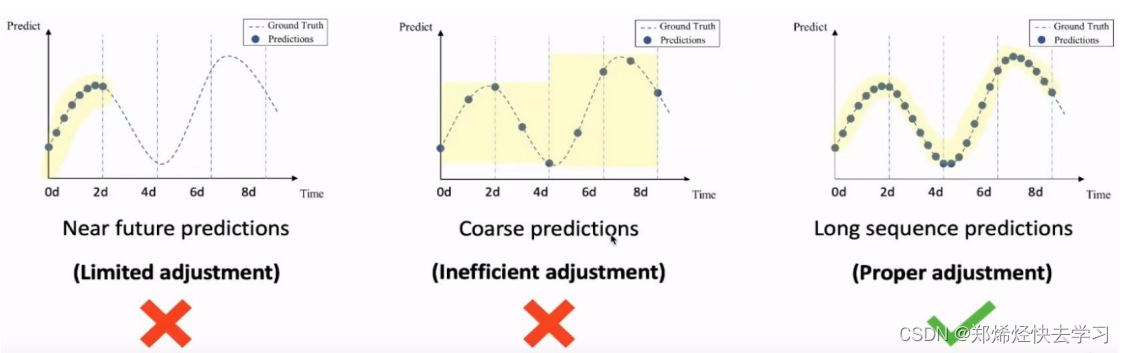
很多算法都是基于短序列进行预测的，先得知前一部分的数据，之后去预测短时间的情况。想要预测一个长序列，就不可以使用短预测，预测未来半年or一年，很难预测很准。长序列其实像是滑动窗口，不断地往后滑动，一步一步走，但是越滑越后的时候，他一直在使用预测好的值进行预测，长时间的序列预测是有难度的。

那么有那些时间序列的经典算法：

• Prophnet：很实用的工具包，很适合 预测趋势，但算的不精准。
• Arima：短序列预测还算精准，但是趋势预测不准。多标签。

当涉及长序列时，上述两种方法都不能使用。

[En]

Neither of the above can be used when long sequences are involved.

• Informer中将主要致力于长序列问题的解决

可能在这里大家也会想到LSTM：但是这个模型在长序列预测中，如果序列越长，那速度肯定越慢，效果也越差。这个模型使用的为串行结构，效率很低，也会基于前面的特征来预测下一个特征，其损失函数的值也会越来越大。

那么我们Transformer中也有提及到改进LSTM的方法，其优势和问题在于：

（1）万能模型，可直接套用，代码实现简单。

（2）并行的，比LSTM快，全局信息丰富，注意力机制效果好。

（3）长序列中attention需要每一个点跟其他点计算，如果序列太长，其效率很低。

（4）Decoder输出很麻烦，都要基于上一个预测结果来推断当前的预测结果，这对于一个长序列的预测中最好是不要出现这样的情况。

那么Informer就需要解决如下的问题：

Transformer的缺点Informer的改进self-attention平方级的计算复杂度提出
ProbSparse Self-attention

筛选出最重要的Q，降低计算复杂度堆叠多层网络，内存占用瓶颈提出
Self-attention Distilling

进行下采样操作，减少维度和网络参数的数量step-by-step解码预测，速度较慢提出
Generative Style Decoder

所有的预测都可以一步到位

[En]

All predictions can be obtained in one step

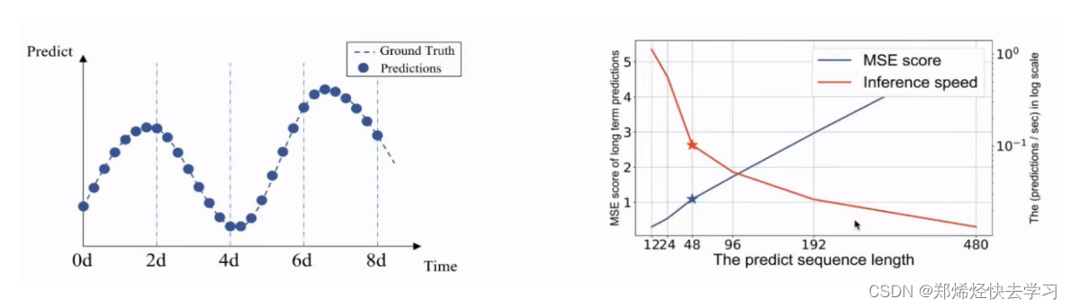
基于以上，Informer提出了LSTF（ Long sequence time-series forecasting）长时间序列预测。

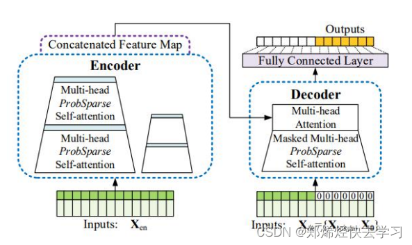
0x03 Informer整体架构

（一）ProbSparse Self-attention

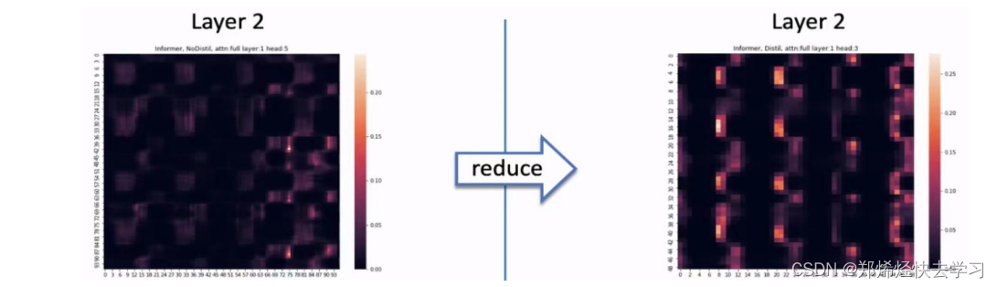
通过以下的数据可以看到，并不是每个QK的点积都是有效值，我们也不需要花很多时间在处理这些数据上：

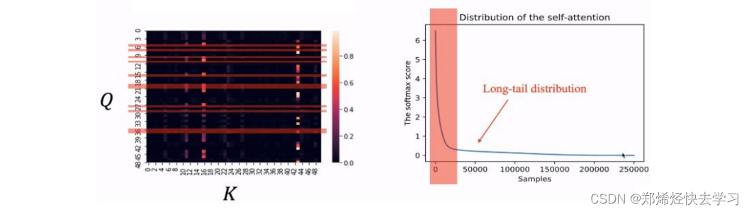
这一结果也是合理的，因为一个元素可能只与几个元素高度相关，而与其他元素没有明显的相关性。如果我们想要提高计算效率，我们需要关注那些特征值，那么我们如何关注这些特征值：

[En]

This result is also reasonable because an element may be highly related to only a few elements and not significantly related to other elements. If we want to improve computational efficiency, we need to pay attention to those characteristic values, then how do we pay attention to those characteristic values:

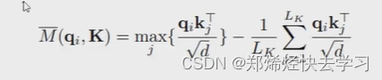
我们需要进行一次Query稀疏性的衡量：

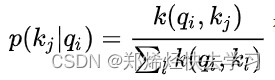
其计算公式如下：

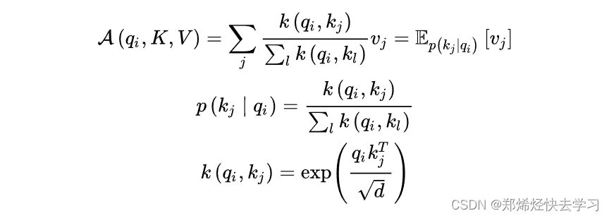
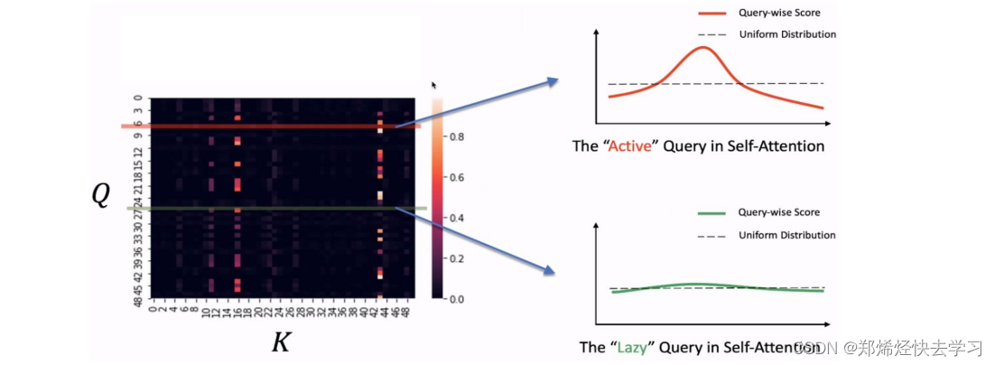
之后我们进行比较：

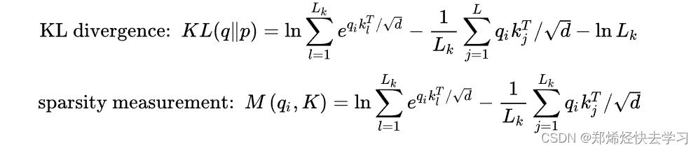
我们算出了其概率以及与均匀分布的差异，如果差异越大，那么这个Q就有机会去被关注、说明其起到了作用。那么其计算方法到底是怎么样进行的，我们要取哪些Q哪些K进行计算:

（1）输入序列长度为96，首先 在K中进行采样，随机选取25个K。

（2）计算每个Q与25个K的点积，可以得到M(qi,K)，现在一个Q一共有25个得分

（3）在25个得分中，选取 最高分的那个Q与均值算差异。

（4）这样我们输入的96个Q都有对应的差异得分，我们将差异从大到小排列，选出差异前25大的Q。

（5）那么传进去参数例如：[32,8,25,96]，代表的意思为输入96个序列长度，32个batch，8个特征，25个Q进行处理。

（6）其他位置淘汰掉的Q使用均匀方差代替，不可以因为其不好用则不处理，需要进行更新，保证输入对着有输出。

以上的时间复杂度为O(L ln L)：
ProbSparse Attention在为每个Q随机采样K时，每个head的采样结果是相同的，也就是采样的K是相同的。但是由于每一层self-attention都会对QKV做线性转换，这使得序列中同一个位置上不同的head对应的QK都不同，那么每一个head对于Q的差异都不同，这就使得每个head中的得到的前25个Q也是不同的。这样也等价于每个head都采取了不同的优化策略。

（二）Self-attention Distilling

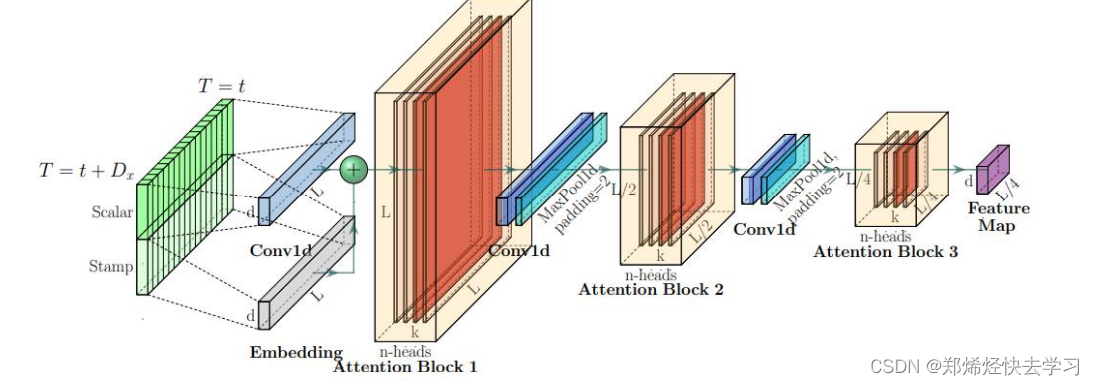
这一层类似于下采样。将我们输入的序列缩小为原来的二分之一。作者在这里提出了自注意力蒸馏的操作，具体是在相邻的的Attention Block之间加入卷积池化操作，来对特征进行降采样。为什么可以这么做，在上面的ProbSparse Attention中只选出了前25个Q做点积运算，形成Q-K对，其他Q-K对则置为0，所以当与value相乘时，会有很多冗余项。这样也可以突出其主要特征，也降低了长序列输入的空间复杂度，也不会损失很多信息，大大提高了效率。

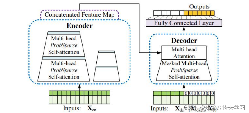
另外，作者为了提高encoder的鲁棒性，还提出了一个strick。途中输入embedding经过了三个Attention Block，最终得到Feature Map。还可以再复制一份具有一半输入的embedding，让它让经过两个Attention Block，最终会得到和上面维度相同的Feature Map，然后把两个Feature Map拼接。作者认为这种方式对短周期的数据可能更有效一些。

（三）Generative Style Decoder

对于Transformer其输出是先输出第一个，再基于第一个输出第二个，以此类推。这样子效率慢并且精度不高。看看总的架构图可以发现，decoder由两部分组成： 第一部分为encoder的输出，第二部分为embedding后的decoder输入，即用0掩盖了后半部分的输入。

看看Embedding的操作：

• Scalar是采用conv1d将1维转换为 512维向量。
• Local Time Stamp采用Transformer中的 Positional Embedding。
• Gloabal Time Stamp则是上述处理后的 时间戳经过Embedding。可以添加上我们的年月日时。

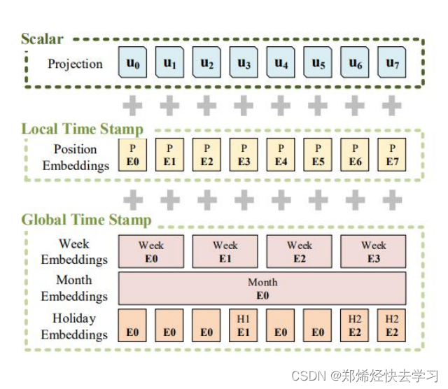
这种位置编码信息具有丰富的回报，不仅包括绝对位置编码，还包括各种时间相关代码。

[En]

This kind of location coding information has a rich return, including not only absolute location coding, but also a variety of time-related codes.

最后，使用三者相加得到相加得到最后的输入(shape:[batch_size,seq_len,d_model])。

Decoder的最后一个部分是过一个linear layer将decoder的输出扩展到与vocabulary size一样的维度上，经过softmax后，选择概率最高的一个word作为预测结果。

那么假设我们有一个已经训练好的Transformer的神经网络，在预测时，传统的步骤是step by step的：

（1）给decoder输入encoder对整个句子embedding的结果和 一个特殊的开始符号。decoder将产生预测，产生”I”。

（2）给decoder输入encoder的embedding结果和”I”，产生预测”am”

（3）给decoder输入encoder的embedding结果和”I am”，产生预测”a”

（4）给decoder输入encoder的embedding的结果和”I am a”，产生预测”student”。

（5）给decoder输入encoder的embedding的结果和”I am a student”，decoder应该生成句子结尾的标记，decoder应该输出” “。

（6）最后decoder生成了，翻译完成。

那么我们再看看Informer一步到位的预测：

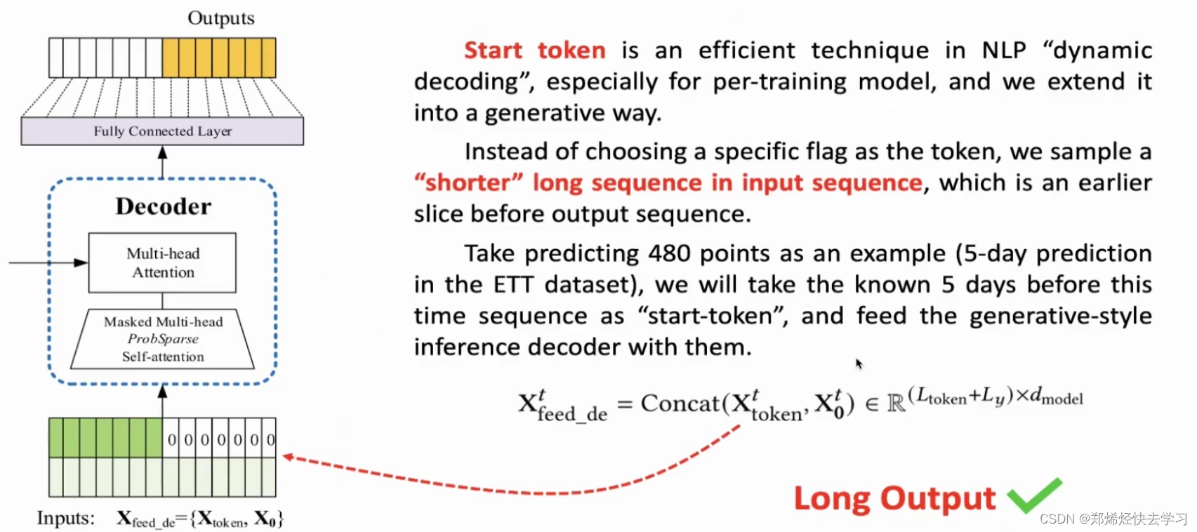
提供一个start标志位：

• 要让Decoder输出预测结果，你得先告诉它从哪开始输出。
• 先给一个引导，比如要输出20-30号的预测结果，Decoder中需先给出。
• 前一序列的结果，例如数字10-20的标签值。
  
  [En]

  the result of the previous sequence, such as the label value of number 10-20.*

对于Decoder输入：

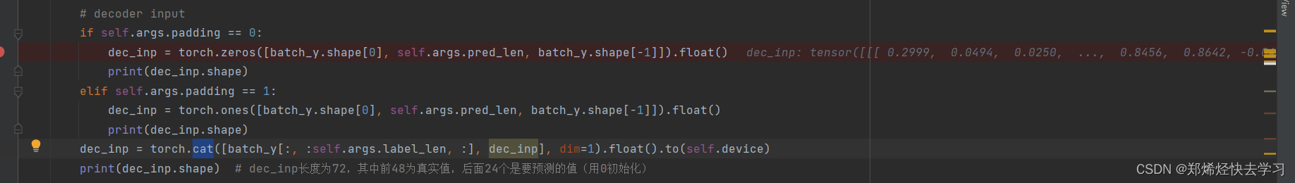
源码中的decoder输入长度为72，其中前48是真实值，后24是预测值。第一步是做自身的ProbAttention，注意要加上Mask（避免未卜先知）。先计算完自身的Attention。再算与encoder的Attention即可。

0x04 计算损失与迭代优化

损失函数为预测值和真值的MSE(均方误差)，并且损失从解码器的输出反向传播到整个模型。优化器使用的Adam。

0x05 源码阅读——站在巨人的肩膀上

（一）环境的搭建

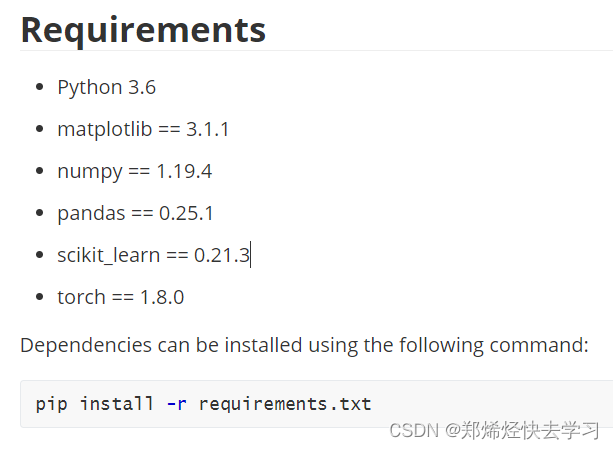
首先我们可以看到Informer所需要的环境：

首先我们需要下载并配置好Anaconda，并下载好PyTorch。安装Anaconda网上很多教程，下面是我安装Pytorch的过程：

• 先配置好清华源

conda config --add channels http://mirrors.tuna.tsinghua.edu.cn/anaconda/pkgs/free/
conda config --add channels http://mirrors.tuna.tsinghua.edu.cn/anaconda/pkgs/main/
conda config --set show_channel_urls yes
conda config --add channels http://mirrors.tuna.tsinghua.edu.cn/anaconda/cloud/pytorch/

如果出现了这种错误：

An HTTP error occurred when trying to retrieve this URL. HTTP errors are often intermittent, and a simple retry will get you on your way.

把镜像源中出现的https改为http就可以了。

清空源的命令：

conda config --remove-key channels

• 创建环境PyTorch

conda create-n pytorch python=3.6

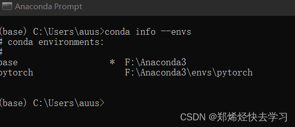
• 查看环境是否安装成功

conda info --envs

• 根据自己的情况安装PyTorch的版本

Pytorch官网：PyTorch

查看自己的CUDA：

nvidia-smi

我的CUDA为11.1，那么安装Pytorch的命令为：

conda install pytorch==1.8.0 torchvision==0.9.0 torchaudio==0.8.0 cudatoolkit=11.1 -c pytorch -c conda-forge

打开Anaconda Prompt命令窗口，进入刚刚所创建的环境中进行

conda activate PyTorch

然后我们就可以进入环境了。

[En]

And then we can get into the environment.

最后，执行官方指令并下载。最后，您可以获得：

[En]

Finally, execute the official instructions and download them. Finally, you can get:

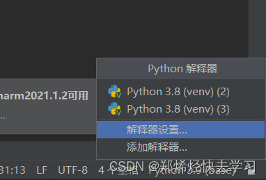
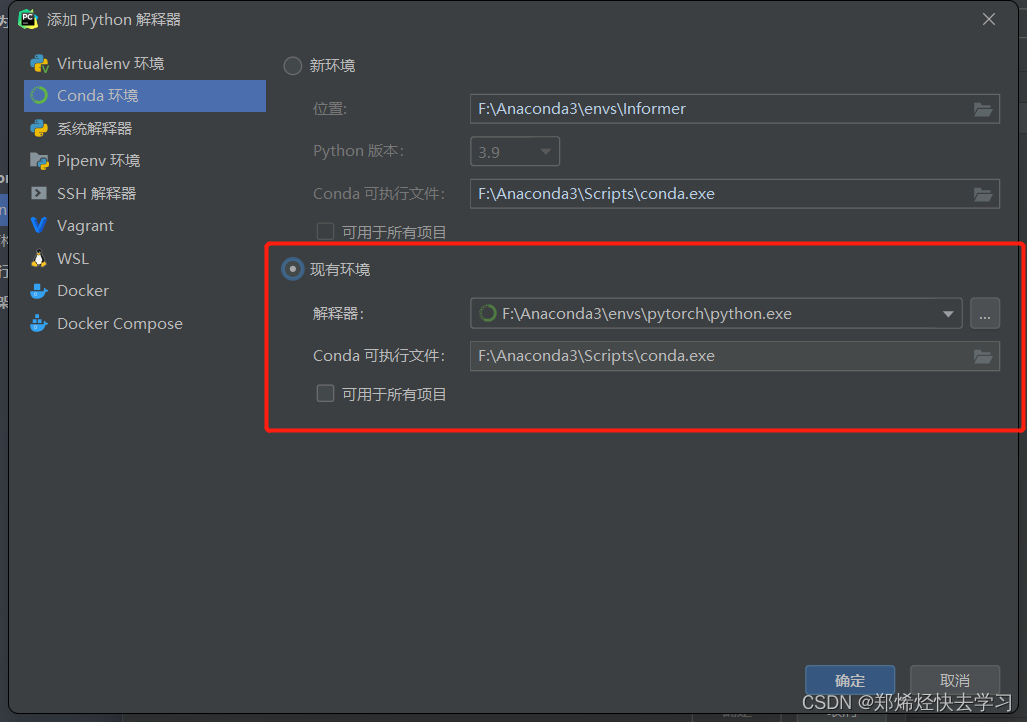
之后进入我们Infomer的源码中进行activate我们的PyTorch环境：

打开PyCharm更改其Python解释器到我们Pytorch文件夹中对应的解释器：

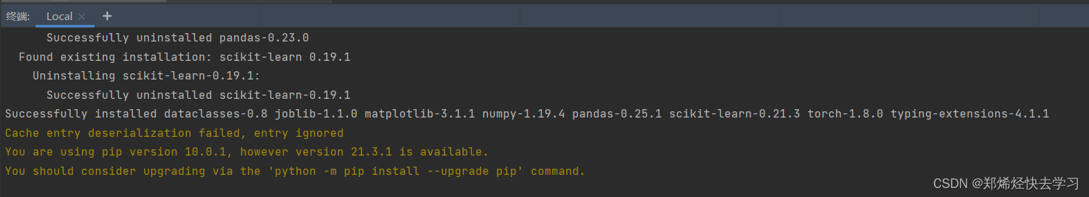
之后在Pycharm的终端中输入：

pip install -r requirements.txt

使用方法：这个项目给了我们三个测试样本，我们只需要输入其中一个：

[En]

How to use it: this project gives us three test samples, and we only need to enter one of them:

ETTh1（指定使用模型为Informer 数据集为哪些 attention机制又为什么 如何处理时间）
python -u main_informer.py --model informer --data ETTh1 --attn prob --freq h

ETTh2
python -u main_informer.py --model informer --data ETTh2 --attn prob --freq h

ETTm1
python -u main_informer.py --model informer --data ETTm1 --attn prob --freq t

然后，我们单击Run查看输出：

[En]

Then we click run to see the output:

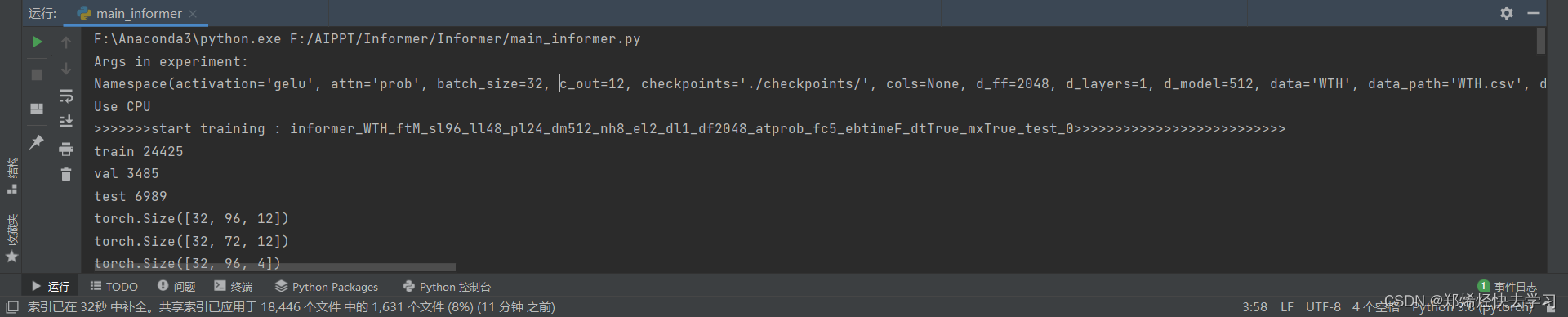
因此，让我们通过断点调试来学习。

[En]

So let’s learn through breakpoint debugging.

（二）Informer文件框架

使用Pycharm打开文件夹我们可以看到如下：

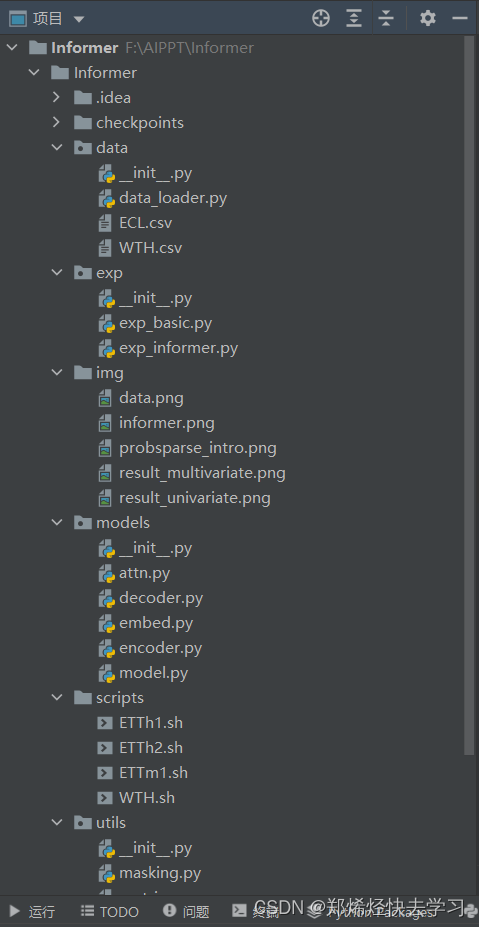
• data

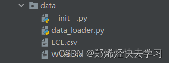
项目的数据文件夹，其中的data_loader文件是加载数据、预处理数据的作用。

• exp

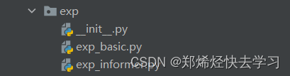
项目训练功能文件夹，这里的py文件是用来训练模型的作用。

• model

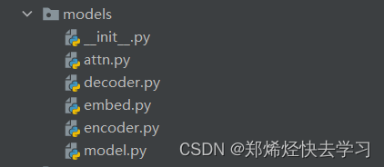
在阅读了上面的一般描述之后，您应该对这些文件要做的事情有了大致的了解。这些都是这个模型的详细实现，所以你可以好好看看。

[En]

After reading the general description above, you should have a general idea of what these files are going to do. these things are the detailed implementation of this model, so you can take a good look.

• scripts

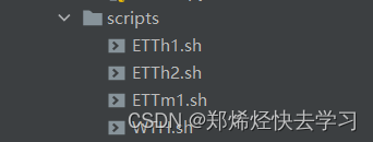
包含模型的启动脚本，使用该脚本。

[En]

Contains the startup script for the model, using the script.

• utils

这里包含了模型的评估指标、时间轴的时间特征处理、指数缩减学习率、提前停止训练策略、数据标准化策略等功能，当然也有Mask机制。

（三）数据的输入

我们打开程序后，我们可以发现有一些数据输入的.csv文件：

这样我们就可以打开源文件，看看它是什么：

[En]

So we can open the source file and see what it is:

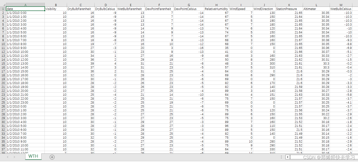
我们可以看到其时间其实是非常明确的，一个样本都有一个固定的时间，我们的数据集是以小时为单位的，可以理解为每个采样点间隔一个小时，后面的内容我们可以理解为一个时间点其具有多个特征，最后的那一列则为输出结果。那么看到这应该可以知道大概怎么替换自己的数据了吧。.csv文件格式适合使用pandas进行处理。

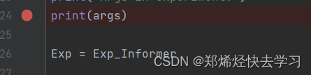
回到main函数，我们在这打上断点1：

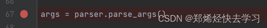
这句话显然是用参数传递的。大多数人可能会看到上面的很多参数，不知道它们是什么，也不知道如何更改它们。我在这里评论了他们中的大多数：

[En]

This sentence is obviously passed in parameters. Most people may see a lot of parameters above and don’t know what they are and how to change them. I have commented most of them here:

parser = argparse.ArgumentParser(description='[Informer] Long Sequences Forecasting')

使用的网络结构（方便对比实验），使用defalut更改网络结构
parser.add_argument('--model', type=str, default='informer',
                    help='model of experiment, options: [informer, informerstack, informerlight(TBD)]')

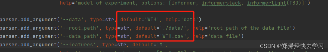
读的数据是什么（类型 路径）
parser.add_argument('--data', type=str, default='WTH', help='data')
parser.add_argument('--root_path', type=str, default='./data/', help='root path of the data file')
parser.add_argument('--data_path', type=str, default='WTH.csv', help='data file')

预测的种类及方法
parser.add_argument('--features', type=str, default='M',
                    help='forecasting task, options:[M, S, MS]; M:multivariate predict multivariate, S:univariate predict univariate, MS:multivariate predict univariate')

哪一列要当作是标签
parser.add_argument('--target', type=str, default='OT', help='target feature in S or MS task')
数据中存在时间 时间是以什么为单位（属于数据挖掘中的重采样）
parser.add_argument('--freq', type=str, default='h',
                    help='freq for time features encoding, options:[s:secondly, t:minutely, h:hourly, d:daily, b:business days, w:weekly, m:monthly], you can also use more detailed freq like 15min or 3h')
模型最后保存位置
parser.add_argument('--checkpoints', type=str, default='./checkpoints/', help='location of model checkpoints')
当前输入序列长度(可定制)<details><summary>*<font color='gray'>[En]</font>*</summary>*<font color='gray'>Current input sequence length (customizable)</font>*</details>
parser.add_argument('--seq_len', type=int, default=96, help='input sequence length of Informer encoder')
标签的长度(具有预测值的东西)(可自定义)<details><summary>*<font color='gray'>[En]</font>*</summary>*<font color='gray'>The length of the label (the thing with the predicted value) (customizable)</font>*</details>
parser.add_argument('--label_len', type=int, default=48, help='start token length of Informer decoder')
预测未来序列长度 （可自定义）
parser.add_argument('--pred_len', type=int, default=24, help='prediction sequence length')
Informer decoder input: concat[start token series(label_len), zero padding series(pred_len)]
编解码器的输入和输出尺寸<details><summary>*<font color='gray'>[En]</font>*</summary>*<font color='gray'>Input and output dimensions of encoder and decoder</font>*</details>
parser.add_argument('--enc_in', type=int, default=7, help='encoder input size')
parser.add_argument('--dec_in', type=int, default=7, help='decoder input size')
输出预测未来多少个值
parser.add_argument('--c_out', type=int, default=7, help='output size')
隐层特征
parser.add_argument('--d_model', type=int, default=512, help='dimension of model')
多头注意力机制
parser.add_argument('--n_heads', type=int, default=8, help='num of heads')
要做几次多头注意力机制
parser.add_argument('--e_layers', type=int, default=2, help='num of encoder layers')
parser.add_argument('--d_layers', type=int, default=1, help='num of decoder layers')
堆叠几层encoder
parser.add_argument('--s_layers', type=str, default='3,2,1', help='num of stack encoder layers')
parser.add_argument('--d_ff', type=int, default=2048, help='dimension of fcn')
对Q进行采样，对Q采样的因子数
parser.add_argument('--factor', type=int, default=5, help='probsparse attn factor')
parser.add_argument('--padding', type=int, default=0, help='padding type')
是否下采样操作pooling
parser.add_argument('--distil', action='store_false',
                    help='whether to use distilling in encoder, using this argument means not using distilling',
                    default=True)
parser.add_argument('--dropout', type=float, default=0.05, help='dropout')
注意力机制
parser.add_argument('--attn', type=str, default='prob', help='attention used in encoder, options:[prob, full]')

parser.add_argument('--embed', type=str, default='timeF',
                    help='time features encoding, options:[timeF, fixed, learned]')
parser.add_argument('--activation', type=str, default='gelu', help='activation')
parser.add_argument('--output_attention', action='store_true', help='whether to output attention in ecoder')
parser.add_argument('--do_predict', action='store_true', help='whether to predict unseen future data')
parser.add_argument('--mix', action='store_false', help='use mix attention in generative decoder', default=True)
读数据
parser.add_argument('--cols', type=str, nargs='+', help='certain cols from the data files as the input features')
windows用户只能给0
parser.add_argument('--num_workers', type=int, default=0, help='data loader num workers')
训练轮数以及epoch
parser.add_argument('--itr', type=int, default=2, help='experiments times')
parser.add_argument('--train_epochs', type=int, default=6, help='train epochs')
parser.add_argument('--batch_size', type=int, default=32, help='batch size of train input data')
停止策略
parser.add_argument('--patience', type=int, default=3, help='early stopping patience')
学习率
parser.add_argument('--learning_rate', type=float, default=0.0001, help='optimizer learning rate')
parser.add_argument('--des', type=str, default='test', help='exp description')
损失函数
parser.add_argument('--loss', type=str, default='mse', help='loss function')
parser.add_argument('--lradj', type=str, default='type1', help='adjust learning rate')
是否为分布式
parser.add_argument('--use_amp', action='store_true', help='use automatic mixed precision training', default=False)
parser.add_argument('--inverse', action='store_true', help='inverse output data', default=False)

parser.add_argument('--use_gpu', type=bool, default=True, help='use gpu')
parser.add_argument('--gpu', type=int, default=0, help='gpu')
parser.add_argument('--use_multi_gpu', action='store_true', help='use multiple gpus', default=False)
如果您指定要分发的多个视频卡<details><summary>*<font color='gray'>[En]</font>*</summary>*<font color='gray'>If you specify several video cards for distribution</font>*</details>
parser.add_argument('--devices', type=str, default='0,1,2,3', help='device ids of multile gpus')

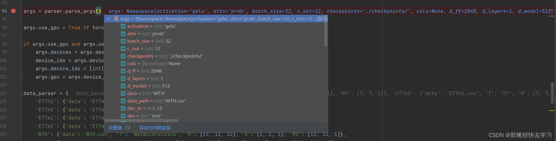
args = parser.parse_args()

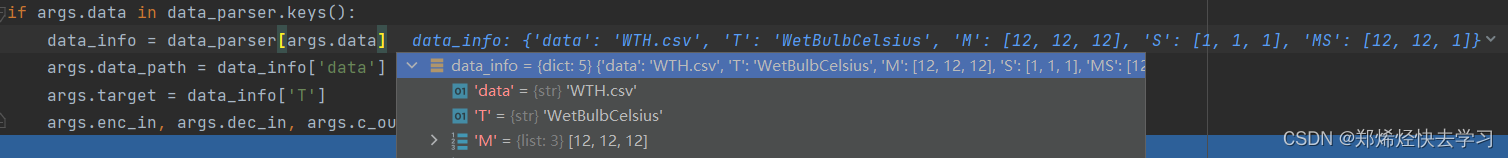
经过单步调试，可以发现上述数据已被读入：

[En]

After single-step debugging, we can find that the above data has been read in:

往下看，我们输入的数据已经定义了几个字典：

[En]

After going down, we can see that the data we entered has been defined as several dictionaries:

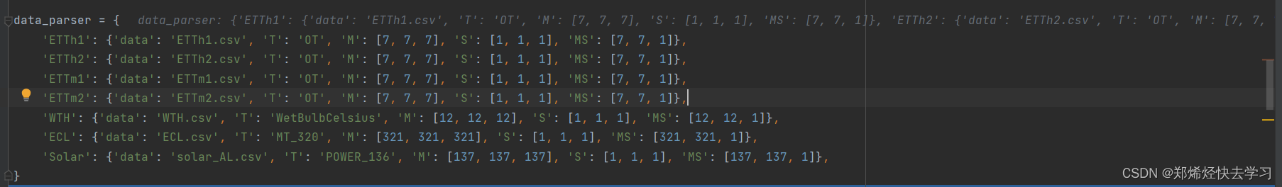
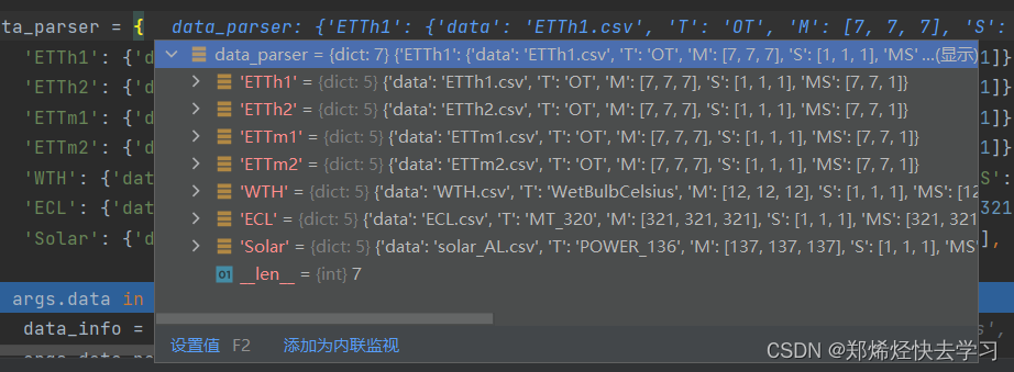
我们可以发现它指定了标签、列、输出大小等等，所以类似地，如果我们想要使用这个模型训练我们自己的数据，我们可以写下：

[En]

We can find that it specifies the label, the column, the output size, and so on, so similarly, if we want to use this model to train our own data, we can write:

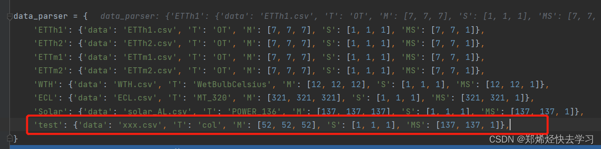
代表的是我在某个csv中读取数据，指定了col列为我的标签，我要预测我未来52个数据。

因此，在此函数中，我们将数据读入我们设置的变量中：

[En]

So in this function, we have read the data into the variables we set:

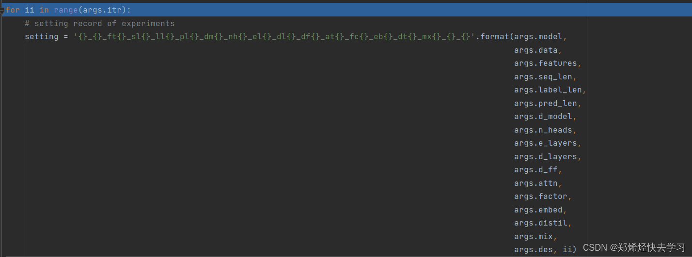
那么下面这个东西也是同理的，我们指定了要循环多少个encoder，时间的频率又是多少，直接从上面读下来：

那么接下来是这样的：

定义一个类。我们存储了我们的数据并开始了培训：

[En]

Defines a class. We stored our data and started training:

我们已经开始重复我们的训练和预测过程：

[En]

We have begun to iterate over our training and forecasting process:

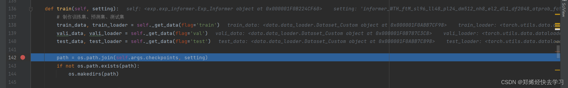
（四）模型训练

（1）预处理

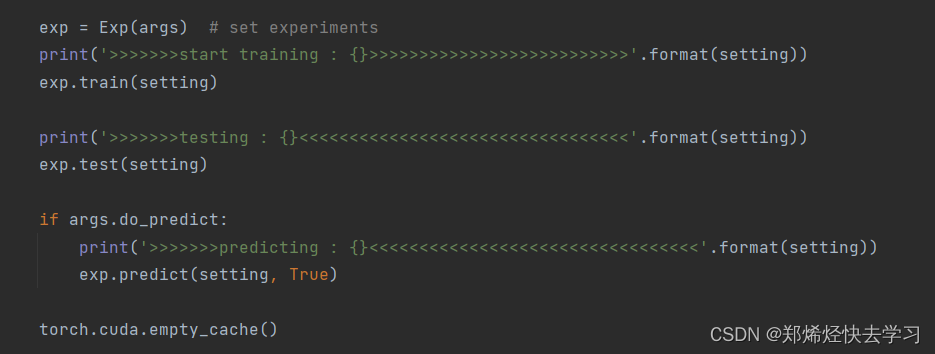
我们跳到它的训练功能，我们可以看到：

[En]

We jump into its training function, and we can see this:

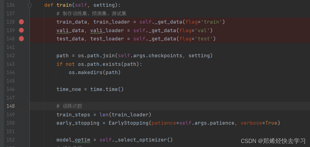
我们可以清楚地看到，上述三个断点是对数据集的划分。让我们先点击训练集：

[En]

We can clearly see that the above three breakpoints are the division of the data set. Let’s click into the training set first:

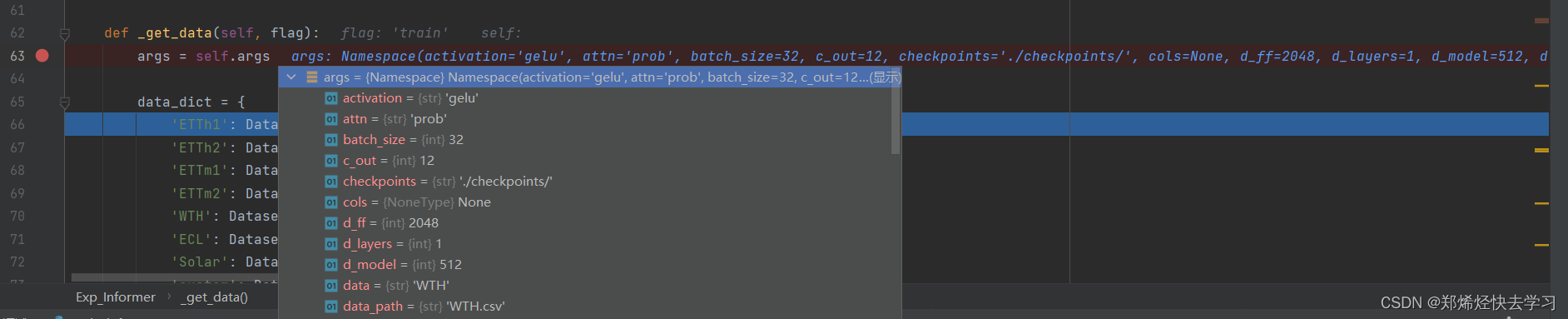
这些其实就是刚刚那个setting中的参数啦。接下来是下面定义的一个字典：

这是我们数据集中的一种数据处理方式，我们可以打开它对应的函数来看看：

[En]

This is a way of dealing with data in our dataset, and we can open its corresponding function to take a look:

在那之后，如何培训那些配置我们数据的人：

[En]

After that, how to train those who configure our data:

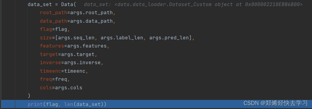
配置完成后，他继续读入数据，并根据配置处理数据：

[En]

After the configuration is completed, he continues to read in the data and process the data according to the configuration:

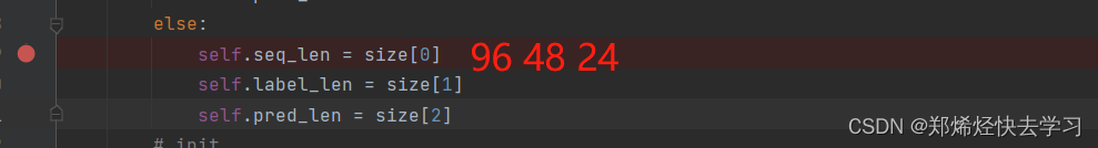
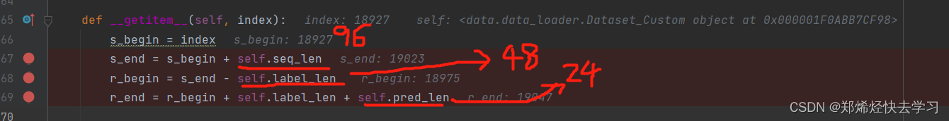
那么当我们进入数据处理的时候，我们可以发现，他把我们要训练的参数，也就是上面的9648和24，划分出了输入序列的长度、有预测的输入值和最终的预测值：

[En]

Well, when we go into the data processing, we can find that he has divided the parameters we want to train, that is, the above 9648 and 24, which delineates the length of the input sequence, the input value with prediction and the final predicted value:

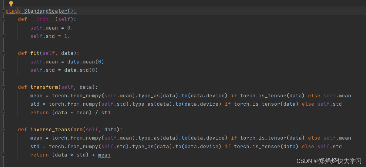
之后是数据标准化处理：

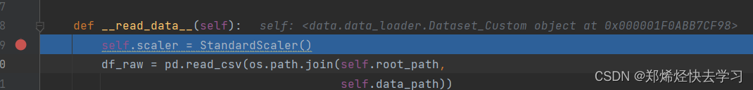
初始化均值和标准差，处理后返回未录入数据的预处理结果。接下来，他开始读入数据：

[En]

Initialize a mean and standard deviation, and return a preprocessing result after processing, at which time no data has been entered. He began to read in the data next:

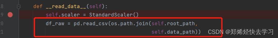
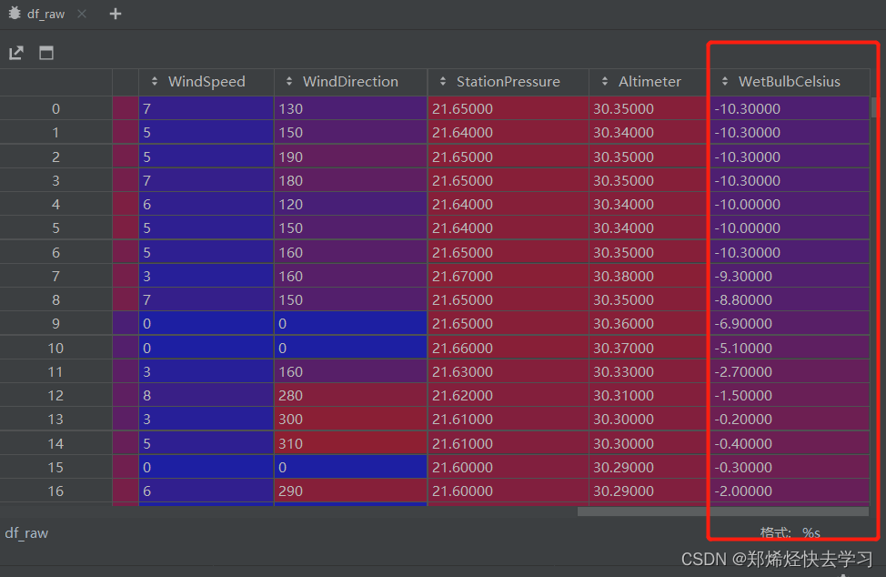
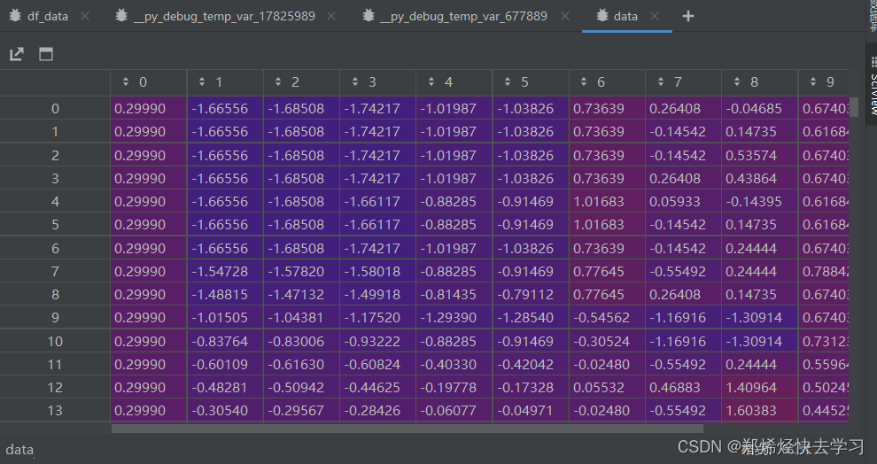
他在这个时候将我们csv的数据都读取了进去，进行标准化操作：

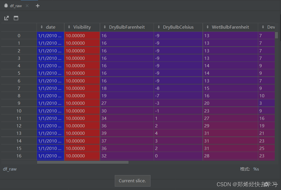
框中的最后一列是我们要预测的标签：

[En]

The last column in the box is the label we want to predict:

接下来就是处理数据了，使用的是 pandas的方法：

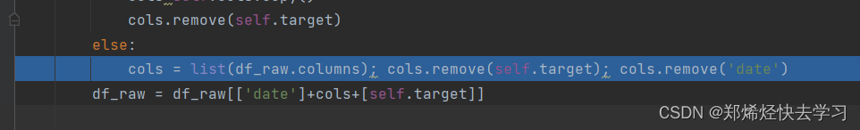
在这一步的时候去除了我们的标签以及日期，因为这些东西并不是我们所要的特征值，所以使用pandas的.columns进行去除。接下来就开始分训练集、测试集以及验证集：

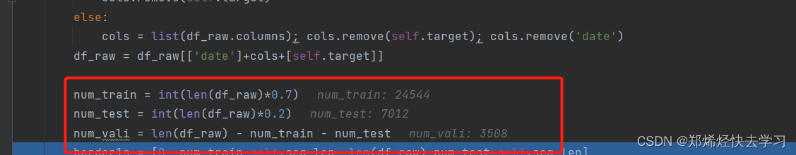
然后，我们指定数据集的开始和结束位置，取出96个序列，取出验证集，并划分训练集、测试集和验证集的位置：

[En]

After that, we specify the start and end position of the data set, take out our 96 sequences, take out our verification set, and divide the location of our training set, test set, and verification set:

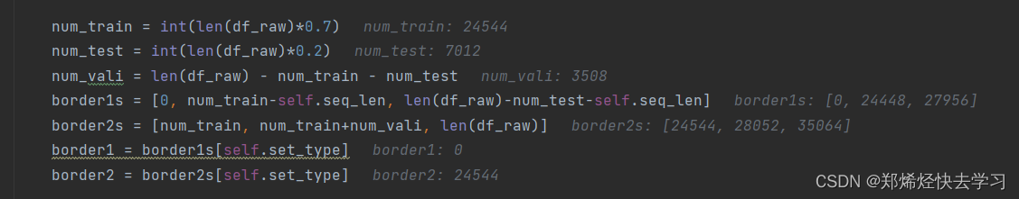
总而言之，上述数字意味着：

[En]

All in all, the above numbers mean this:

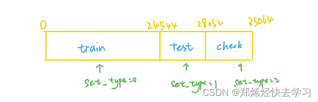
我们就可以根据前面的set_type变量来设定我们的边界。

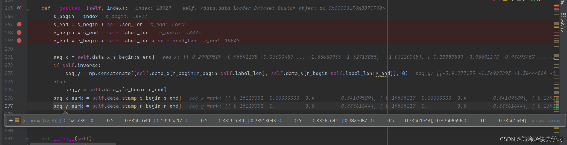
在这一步中，我们移走了我们面前的时间，留下了我们所有的特征：

[En]

In this step, we remove the time in front of us and leave all our characteristics:

之后我们就进行标准化操作了，我们先将我们训练集的数据拿进去算均值以及方差，最后再进行transformer操作：

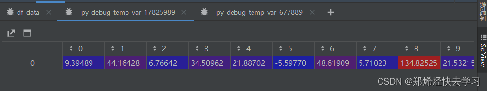
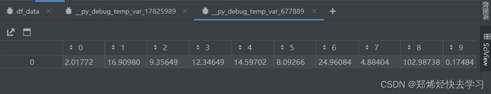
最后，每个数字可以得到一个数据，即每个数字的标准差减去它的平均值，然后除以方差，这是一个非常基本的标准化运算：

[En]

Finally, each number can get a data, which is a standard deviation of each number minus its mean and then divided by variance, which is a very basic standardized operation:

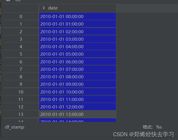
之后我们再分离出我们的时间，时间序列的训练肯定少不了很多时间的处理方式，最后转换为pandas的格式，方便pandas的处理：

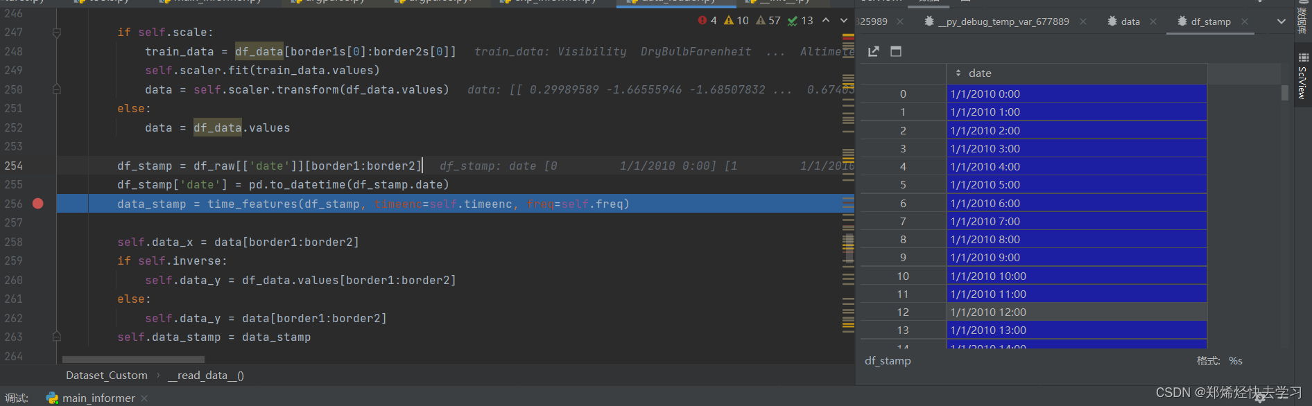
关于时间的处理：

看看这个东西：

return np.vstack([feat(dates) for feat in time_features_from_frequency_str(freq)]).transpose(1,0)

先看看函数time_features_from_frequency_str：

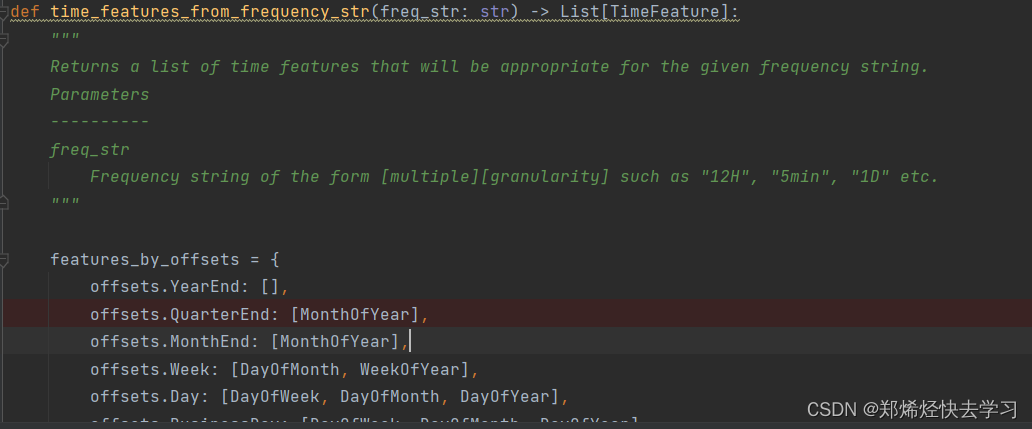
这实际上是我们前面谈到的特征提取，它以几个小时为单位，返回适合给定频率字符串的时间特征列表。

[En]

This thing is actually the feature extraction that we talked about earlier, which takes several hours as a unit, and * returns a list of time features suitable for a given frequency string.*

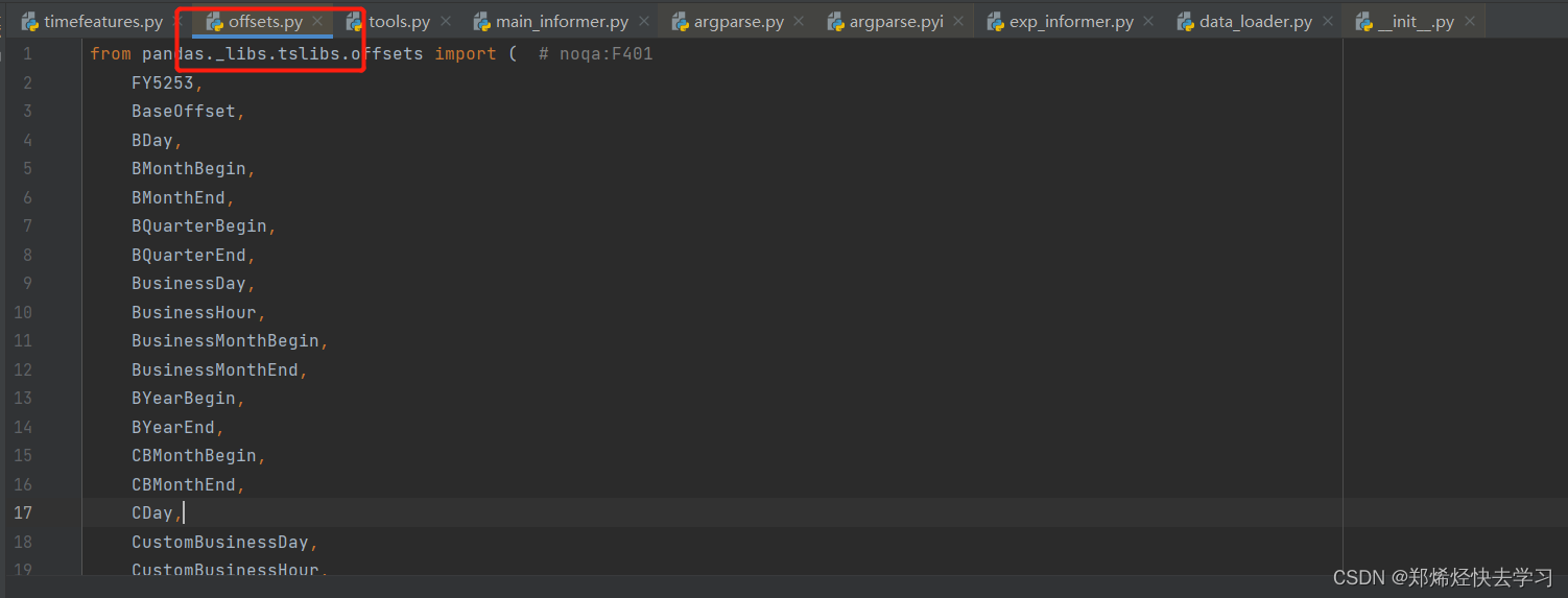
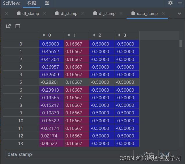
那么里面offsets又是什么东西，其实就是pandas已经处理好的包了，它的目的是想将我们csv中的时间，根据日月年时间进行读取特征，并且用其他数字来代替这些时间，我们可以看看具体的操作。

class SecondOfMinute(TimeFeature):
    """Minute of hour encoded as value between [-0.5, 0.5]"""
    def __call__(self, index: pd.DatetimeIndex) -> np.ndarray:
        return index.second / 59.0 - 0.5

class MinuteOfHour(TimeFeature):
    """Minute of hour encoded as value between [-0.5, 0.5]"""
    def __call__(self, index: pd.DatetimeIndex) -> np.ndarray:
        return index.minute / 59.0 - 0.5

class HourOfDay(TimeFeature):
    """Hour of day encoded as value between [-0.5, 0.5]"""
    def __call__(self, index: pd.DatetimeIndex) -> np.ndarray:
        return index.hour / 23.0 - 0.5

class DayOfWeek(TimeFeature):
    """Hour of day encoded as value between [-0.5, 0.5]"""
    def __call__(self, index: pd.DatetimeIndex) -> np.ndarray:
        return index.dayofweek / 6.0 - 0.5

class DayOfMonth(TimeFeature):
    """Day of month encoded as value between [-0.5, 0.5]"""
    def __call__(self, index: pd.DatetimeIndex) -> np.ndarray:
        return (index.day - 1) / 30.0 - 0.5

class DayOfYear(TimeFeature):
    """Day of year encoded as value between [-0.5, 0.5]"""
    def __call__(self, index: pd.DatetimeIndex) -> np.ndarray:
        return (index.dayofyear - 1) / 365.0 - 0.5

class MonthOfYear(TimeFeature):
    """Month of year encoded as value between [-0.5, 0.5]"""
    def __call__(self, index: pd.DatetimeIndex) -> np.ndarray:
        return (index.month - 1) / 11.0 - 0.5

class WeekOfYear(TimeFeature):
    """Week of year encoded as value between [-0.5, 0.5]"""
    def __call__(self, index: pd.DatetimeIndex) -> np.ndarray:
        return (index.isocalendar().week - 1) / 52.0 - 0.5

最后处理后的时间如下：

[En]

The time after the final processing is as follows:

这就是我们所有的数据处理。并且训练集、测试集、验证集都是相同的。到目前为止，我们的训练集、测试集和验证集都已经完成：

[En]

So that’s all our data processing. And the training set, the test set, the verification set are all the same. So by now, our training set, test set, and verification set have all been done:

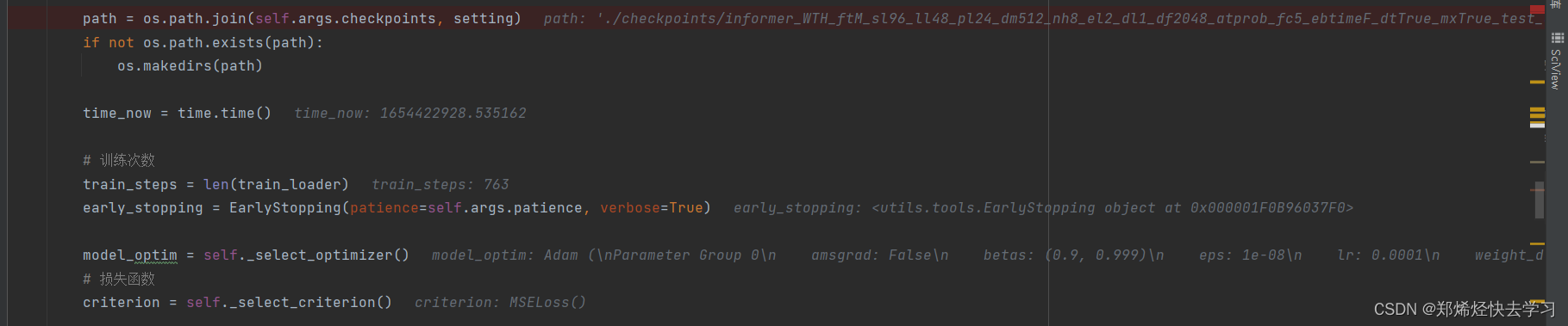
之后，训练开始，定义了模型的位置、计算时间、训练次数和损失函数的定义：

[En]

After that, the training began, defining the location of the model, the calculation time, the number of training and the definition of the loss function:

每次迭代进入此函数进行数据处理：

[En]

Each iteration enters this function for data processing:

在这里他对96个输入作为x，将72个输出作为y：

那么以上循环32次。

（2）encoder

接下来看看 模型的搭建：

在decoder的处理中，我们先将decoder输入预测的24个值全部初始化为0，之后再进行拼接：

最后，我们将把上面处理过的值传递到网络结构中：

[En]

So finally, we’re going to pass the values we handled above into the network structure:

• batch_x与batch_x_mark：输入的encoder的数据，96个长度以及96个数据的时间
• dec_inp与batch_y_mark：输出的decoder的数据，72个数据以及72个数据的时间

模型的搭建位于model.py中的Informer类中：

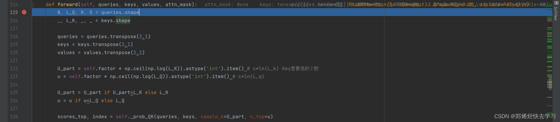
我们首先看看forward函数：

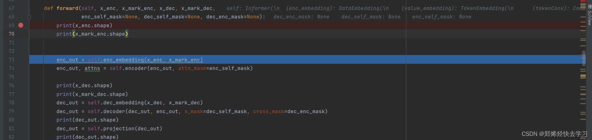
对于输入的函数，我们首先进行了embeddding，是什么操作？

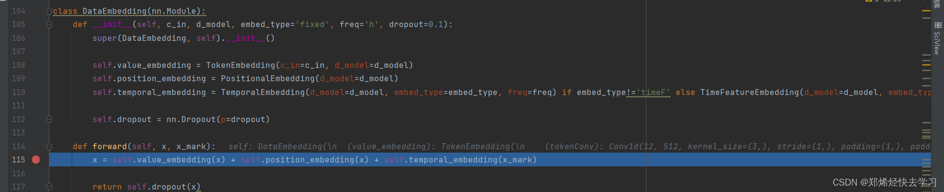
对输入的序列进行一维卷积，并且使用padding等操作后，最后变为512维的向量：

之后，添加位置编码和时间特征，它们最多映射到512个特征。

[En]

After that, position coding and time features are added, which are most mapped to 512 features.

最后的x是这样的：

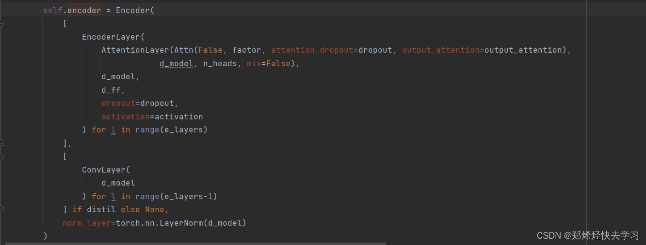
class Encoder(nn.Module):
    def __init__(self, attn_layers, conv_layers=None, norm_layer=None):
        super(Encoder, self).__init__()
        self.attn_layers = nn.ModuleList(attn_layers)
        self.conv_layers = nn.ModuleList(conv_layers) if conv_layers is not None else None
        self.norm = norm_layer

    def forward(self, x, attn_mask=None):
        # x [B, L, D]
        attns = []
        if self.conv_layers is not None:
            for attn_layer, conv_layer in zip(self.attn_layers, self.conv_layers):
                x, attn = attn_layer(x, attn_mask=attn_mask)
                x = conv_layer(x) # pooling后再减半，还是为了速度考虑
                attns.append(attn)
            x, attn = self.attn_layers[-1](x, attn_mask=attn_mask)
            attns.append(attn)
        else:
            for attn_layer in self.attn_layers:
                x, attn = attn_layer(x, attn_mask=attn_mask)
                attns.append(attn)

        if self.norm is not None:
            x = self.norm(x)

        return x, attns

之后我们跳进去EncoderLayer中：

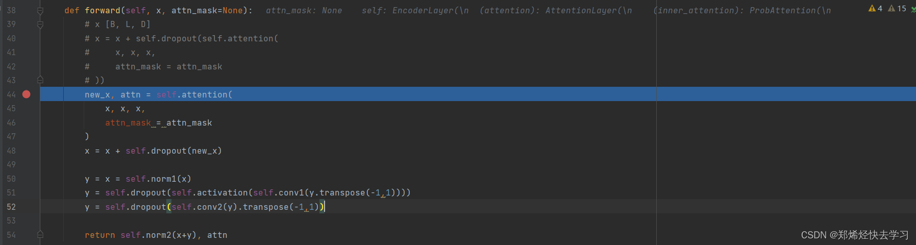
我们发现其输入了3个x，为什么要三个x？原因是我们想要计算QKV矩阵呀。之后我们就步入了AttentionLayer：

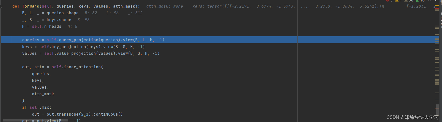
我们将我们输入的参数x，分别乘以三个权重参数矩阵，可以得到QKV三个向量。在这一步也同样做了多头注意力机制的操作，在上面定义了8个头，在view的过程中将其转换为512=8*64，形成了多头注意力机制。

之后进入了Informer独有的 ProbAttention：

也就是上面所说的，筛选出明显特征的Q，找出Q的代表！！这篇论文最核心的东西了。

这里计算出了我们需要25个Q：

之后进入了 _prob_QK：

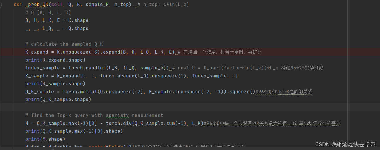
它先将K进行复制，扩充了一个维度，之后进行随机采样25个K。再使用25个K与96个Q相乘计算其内积。最后得到的是96*25的的矩阵，最后再赋予到那个复制的维度中。之后我们再继续算出了Q与K之间的关系：

首先找出每一个Q（一共96个Q）中最大的那个值，之后要与均匀分布作比较：

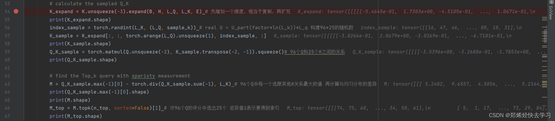
比较完后，我们进行排序，最后得到索引，去找对应的25个Q。

到了这里，我们已经采样完25个特征最明显的Q了。K还是一样保持了96个。这样我们的ProAttention就这么算完了。

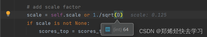
之后再排除掉维度造成的影响，也就是公式中除的那个根号d：

之后我们要对V矩阵进行处理，我们进入到函数 _get_initial_context：

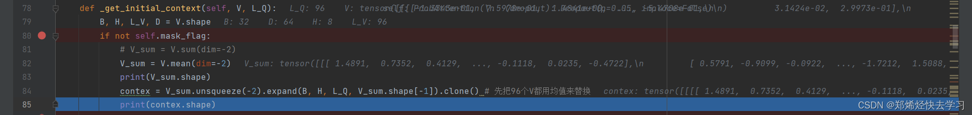
在这里我们将没有视为特征的Q，使用均值来代替。让他一直在平庸。在这一步我们还没有得知25个Q是哪些，我们把所有的V都初始化为我们的平庸值。

之后我们将有特征的值进行保留，进入函数 _update_context：

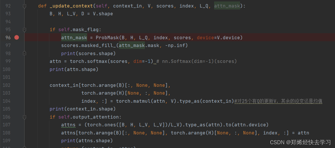
在其中，我们也执行了softmax操作，目的是为了这条公式：

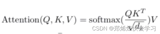
之后我们对25个Q进行更新V，并且计算好了其Attention。之后返回了我们的上下文，并且经过了全连接。

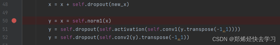
（3）dropout

这个操作就是Transformer中的残差连接。叫做 至少不比原来差。

（4）Convlayer

蒸馏操作，我们需要做多次attention，但是我们不会以原大小进行操作，我们会将其缩小为原来的二分之一，提速的作用：1维卷积+ELU激活函数+最大池化

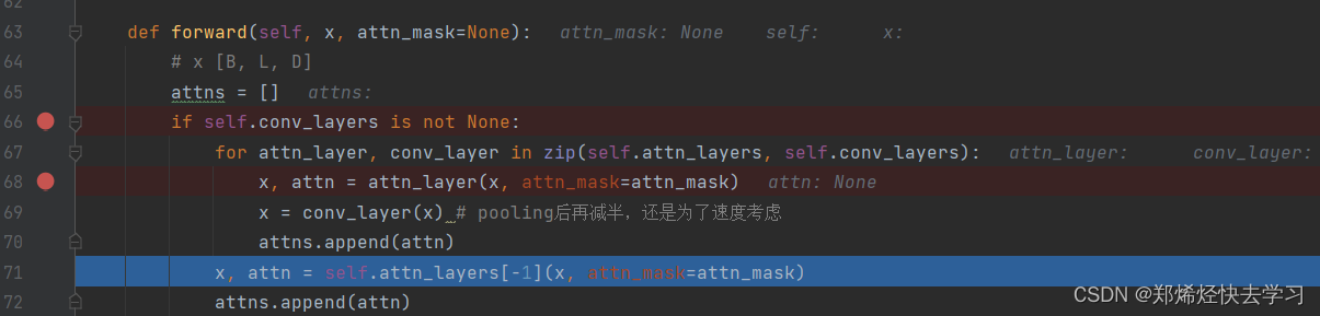
然后重复我们上面所做的。

[En]

Then repeat what we did above.

（5）decoder

以上我们就已经执行完了encoder的操作了，短短的两行程序操作了很多东西：

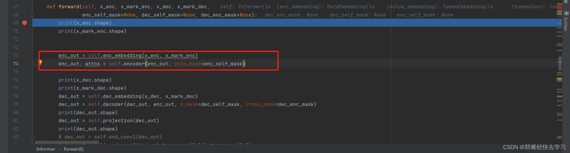
那么我们就进入decoder的世界了：

首先我们进行了embedding，这个操作跟上面的是一模一样的。

之后进入了类Decoder：

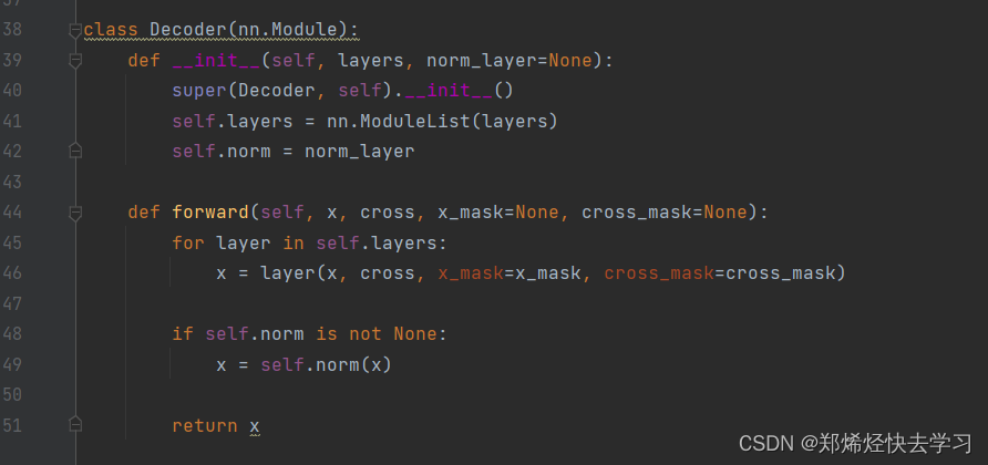
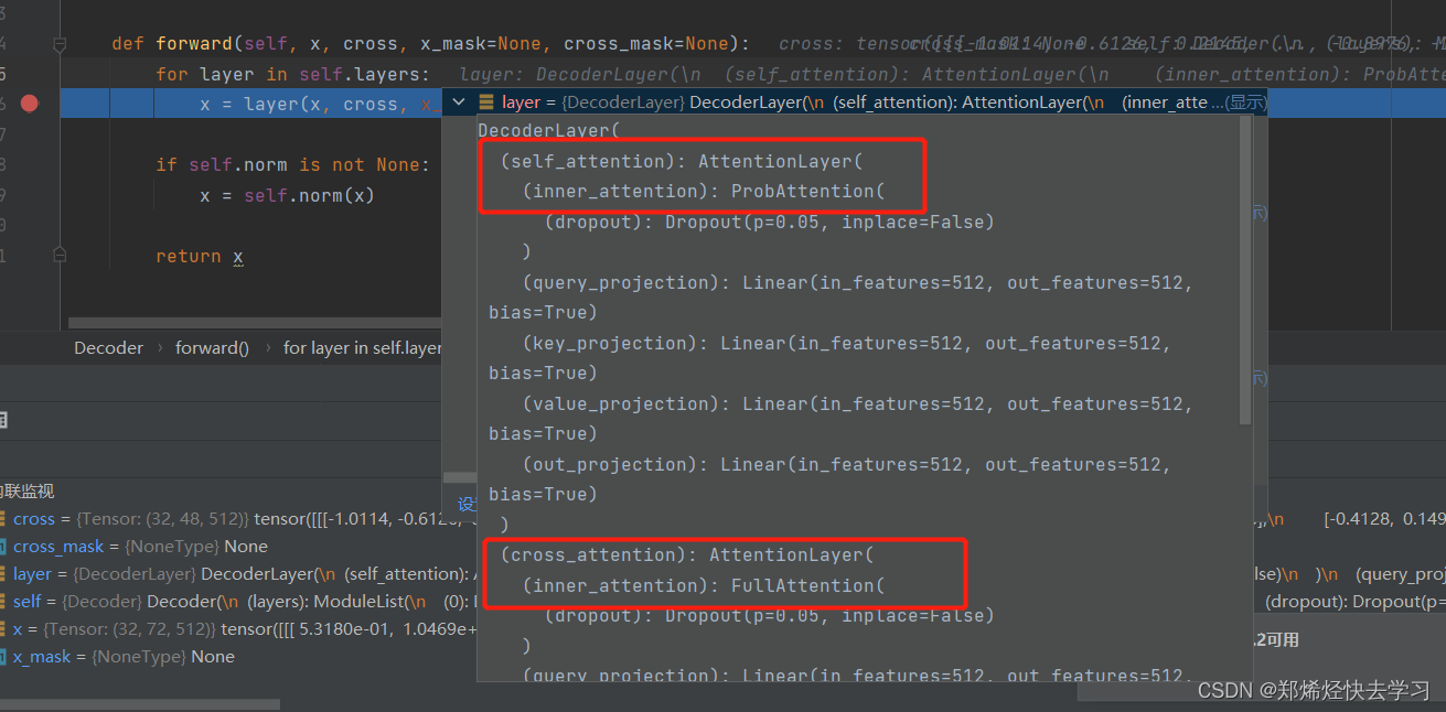
我们可以发现上面框住的Attention与下面的那个框其实是不一样的，但是上面的那个执行过程，与encoder其实是一模一样的。

不一样在哪呢，我们的decoder加入了mask机制呀，最大的区别就是不可以未卜先知。也就是图示中的Masked Multi-head。

那么我们进入FullAttention去看看操作到底是怎么样的：

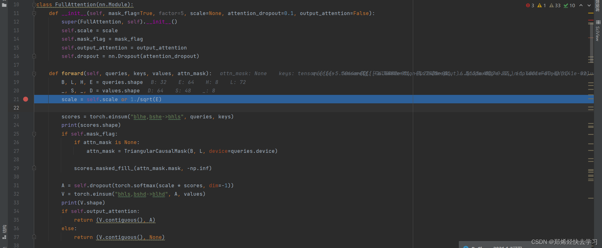
那么self-attention与cross-attention有什么区别呢：

• self-attention是自己与自己之间
• cross-attention是encoder与decoder之间

其他一切都是一样的。

[En]

Everything else is exactly the same.

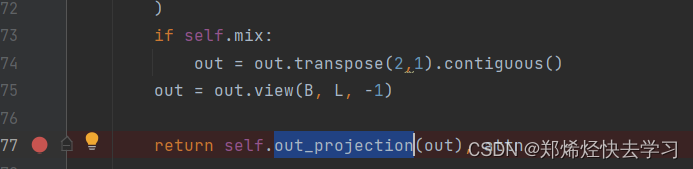
那么从代码中我们可以发现，我们最后的输出是联系了encoder的self-attention以及decoder的cross-attention：

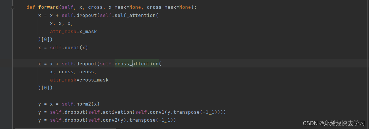
上面的self-attention中，输入的三个x其实是为了计算我们的QKV，这个x其实就是我们那96个从csv文件中读取出来的数据，而下面的cross-attention，首先输入的第一个x是我们decoder前embedding好的要带着我们预测数据的那48个值，它只需要一个Q向量，我们使用encoder中算出来的Ek以及Ev进行预测我们要的预测值。

然后再做一次剩余的连接，然后我们就要赢了！

[En]

And then make another residual connection, and then we’re about to win!

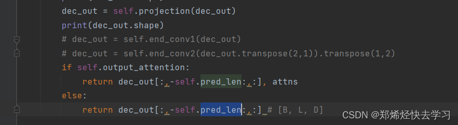
之后我们对我们的72个输出，将48个进行抛弃，读取我们需要的24个。并且这个模型做了一个多变量的预测。需要注意的是，Mask机制只是将48个后面的24个进行mask，而不是一开始就直接mask。

我花了很多时间来学习这个网络。我希望我下次能更有效率！

[En]

It took me a lot of time to learn this network. I hope I can be more efficient next time!

Original: https://blog.csdn.net/Alkaid2000/article/details/125137982
Author: 郑烯烃快去学习
Title: 源码阅读及理论详解《 Informer: Beyond Efficient Transformer for Long Sequence Time-Series Forecasting 》