

Adaboost分类算法原理及代码实例
- 一、Adaboost 简介
- 一、Adaboost 算法过程
- 二、简单实例
- 三、python 实现
* - 3.1 sklearn.AdaBoostClassifier 参数说明
- 3.2 导入相关库与数据集
- 3.3 划分训练集、预测集
- 3.4 Adaboost模型训练
- 3.5 模型预测与评价
一、Adaboost 简介
集成学习(Ensemble Learning) 是机器学习领域表现最强的一大分支,主要原理是将多个弱机器学习器结合,构建一个有较强性能的机器学习器。集成学习方法可以分为两类: Boosting 和 Bagging。
Bagging:它的特点是各个弱学习器是并行关系,相互之间没有依赖,如随机森林算法,是由多个独立决策树模型共同组成。
Boosting, 也称为增强学习或提升法,特点是当前的弱学习器与上一弱学习器之间有依赖关系,且可以通过不断地构建多个”链式”弱学习器,最终形成一个强学习器。
AdaBoost 属于Boosting算法的一种,英文全称”Adaptive Boosting”(自适应增强),它的自适应在于: 前一个基本分类器被错误分类的样本的权值会增大,而正确分类的样本的权值会减小,并再次用来训练下一个基本分类器。同时,在每一轮迭代中,加入一个新的弱分类器,直到达到某个预定的足够小的错误率或达到预先指定的最大迭代次数才确定最终的强分类器。


; 一、Adaboost 算法过程
- 给定一个二分类数据集
T = { ( x 1 , y 1 ) , ( x 2 , y 2 ) , . . . , ( x N , y N ) } T = { (x_{1},y_{1}),(x_{2},y_{2}),…,(x_{N},y_{N}) }T ={(x 1 ,y 1 ),(x 2 ,y 2 ),…,(x N ,y N )}
其中,y i ∈ { − 1 , 1 } y_{i} \in { -1,1 }y i ∈{−1 ,1 } - 算法流程:
(1)初始化每条数据的权重
D 1 = ( w 1 , w 2 , . . . , w N ) = ( 1 N , 1 N , . . . , 1 N ) D_{1} = (w_{1},w_{2},…,w_{N}) = (\frac{1}{N},\frac{1}{N},…,\frac{1}{N})D 1 =(w 1 ,w 2 ,…,w N )=(N 1 ,N 1 ,…,N 1 )
(2)进行迭代
a. 选取一个误差率最低的弱分类器 h h h 作为第 t t t 个基分类器 h t h_{t}h t ,并计算该基分类器的拟合误差率:
e t = P ( h t ( x i ) ≠ y i ) = ∑ i = 1 N w t i I ( h t ( x i ) ≠ y i ) e_{t} = P(h_{t}(x_{i}) \neq y_{i}) = \sum_{i=1}^{N}{w_{ti} I(h_{t}(x_{i}) \neq y_{i})}e t =P (h t (x i )=y i )=i =1 ∑N w t i I (h t (x i )=y i )
其中,I ( h t ( x i ) ≠ y i ) = { 0 , h t ( x i ) = y i 1 , h t ( x i ) ≠ y i I(h_{t}(x_{i}) \neq y_{i})= \begin{cases} 0, &h_{t}(x_{i}) = y_{i} \ 1, &h_{t}(x_{i}) \neq y_{i} \end{cases}I (h t (x i )=y i )={0 ,1 ,h t (x i )=y i h t (x i )=y i
不难看出,拟合误差率其实就是误分类样本的权值之和。
b. 计算基分类器h t h_{t}h t 在最终分类器H H H中所占的权重
α t = 1 2 l n ( 1 − e t e t ) \alpha_{t} = \frac{1}{2} ln(\frac{1-e_{t}}{e_{t}})αt =2 1 l n (e t 1 −e t )
c. 更新样本权重D t + 1 D_{t+1}D t +1
D t + 1 = D t e x p ( − α t y i h t ( x i ) ) Z t D_{t+1} = \frac { D_{t} exp(- \alpha_{t} y_{i} h_{t}(x_{i})) } { Z_{t} }D t +1 =Z t D t e x p (−αt y i h t (x i ))
其中,Z t Z_{t}Z t 是归一化常数,Z t = 2 e t ( 1 − e t ) Z_{t} = 2 \sqrt{e_{t}(1-e_{t})}Z t =2 e t (1 −e t )
从样本权重更新公式可以看出,权重更新依赖于α t \alpha_{t}αt ,且α t \alpha_{t}αt 依赖于e t e_{t}e t ,所以更新公式可以简化成:
当样本分类错误时,y i h t ( x i ) = − 1 y_{i} h_{t}(x_{i}) = -1 y i h t (x i )=−1
D t + 1 = D t 2 e t D_{t+1} = \frac{D_{t}}{2e_{t}}D t +1 =2 e t D t
当样本分类正确时,y i h t ( x i ) = − 1 y_{i} h_{t}(x_{i}) = -1 y i h t (x i )=−1
D t + 1 = D t 2 ( 1 − e t ) D_{t+1} = \frac{D_{t}}{2(1-e_{t})}D t +1 =2 (1 −e t )D t
关于Z t Z_{t}Z t 与D t + 1 D_{t+1}D t +1 的推导说明参考:Adaboost算法原理分析和实例+代码(简明易懂)
(3)最后,让每个弱分类器h t h_{t}h t 与权重α t \alpha_{t}αt 进行组合
f ( x ) = ∑ α t h t f(x) = \sum {\alpha_{th_{t}}}f (x )=∑αt h t
通过符号函数s i g n ( ) sign()s i g n (),可以得到最终的强分类器
H = s i g n ( f ( x ) ) H = sign(f(x))H =s i g n (f (x ))
综上所述,构建最终的分类器迭代过程可以写成
H t = H t − 1 + α t h t H_{t} = H_{t-1} +\alpha_{t}h_{t}H t =H t −1 +αt h t
我们可以加一个迭代速率β \beta β,控制迭代快慢
H t = H t − 1 + β α t h t H_{t} = H_{t-1} +\beta \alpha_{t}h_{t}H t =H t −1 +βαt h t
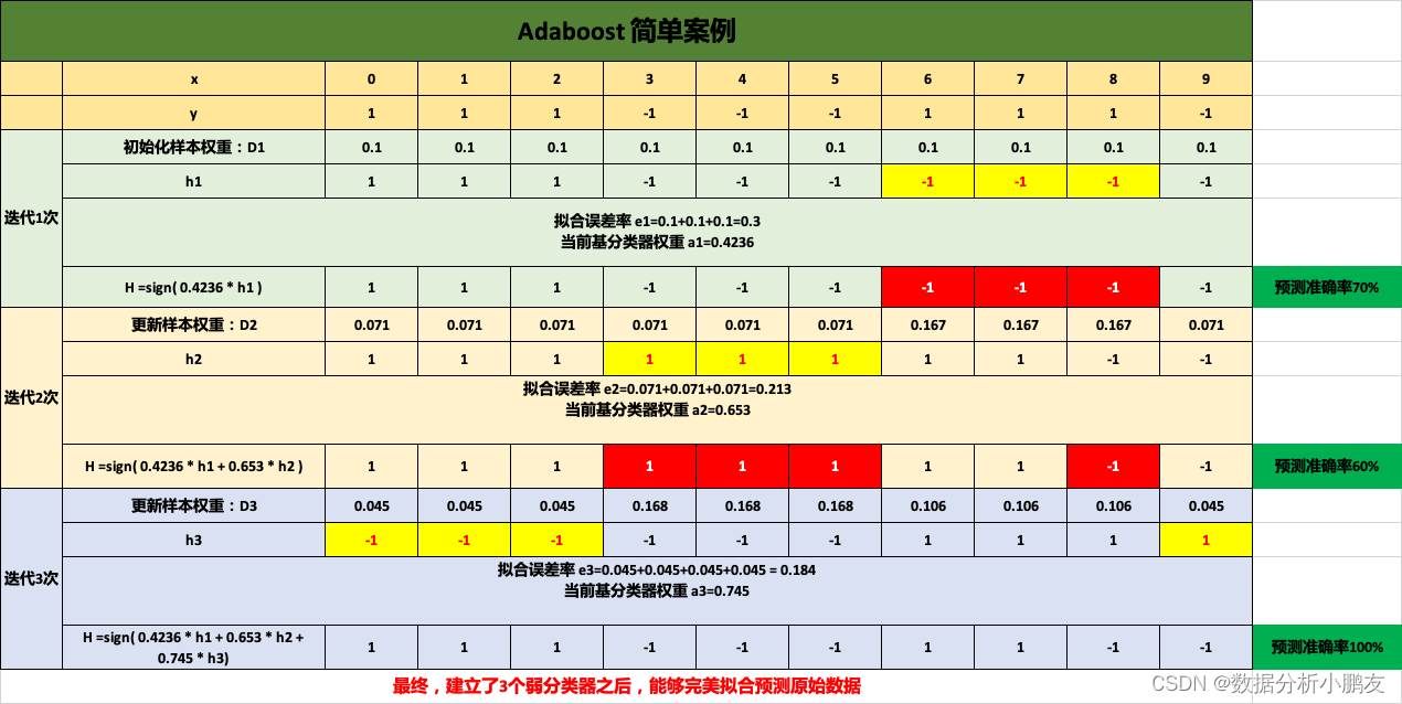
二、简单实例
- 给定一个简单的二分类数据集

- 算法过程
(1)初始化每条数据的权重
此处N=10.
D 1 = ( w 1 , w 2 , . . . , w 10 ) = ( 1 10 , 1 10 , . . . , 1 10 ) D_{1} = (w_{1},w_{2},…,w_{10}) = (\frac{1}{10},\frac{1}{10},…,\frac{1}{10})D 1 =(w 1 ,w 2 ,…,w 10 )=(10 1 ,10 1 ,…,10 1 )
(2)迭代第1次
a. 选取一个误差率最低的弱分类器 h h h 作为第 1 1 1 个基分类器 h 1 h_{1}h 1 ,并计算该基分类器的拟合误差率:h 1 = { 1 , x < 2.5 − 1 x > = 2.5 h_{1}= \begin{cases} 1, & x < 2.5 \ -1 & x >= 2.5 \end{cases}h 1 ={1 ,−1 x <2.5 x >=2.5 ,得到的结果是[ 1,1,1,-1, -1,-1,-1,-1,-1,-1],能够发现x为6,7,8的数据结果分类错误,计算得到其错误率为:
e 1 = 0.1 + 0.1 + 0.1 = 0.3 e_{1} = 0.1 + 0.1 +0.1 = 0.3 e 1 =0.1 +0.1 +0.1 =0.3
b. 计算基分类器h 1 h_{1}h 1 在最终分类器H H H中所占的权重
α 1 = 1 2 l n ( 1 − e 1 e 1 ) = 0.4236 \alpha_{1} = \frac{1}{2} ln(\frac{1-e_{1}}{e_{1}}) = 0.4236 α1 =2 1 l n (e 1 1 −e 1 )=0.4236
c. 更新样本权重D 2 D_{2}D 2
当样本分类错误时,D 2 = D 1 2 e 1 = 0.071 D_{2} = \frac{D_{1}}{2e_{1}} = 0.071 D 2 =2 e 1 D 1 =0.071;当样本分类正确时,D 2 = D 1 2 ( 1 − e 1 ) = 0.167 D_{2} = \frac{D_{1}}{2(1-e_{1})} = 0.167 D 2 =2 (1 −e 1 )D 1 =0.167。
d. 得到第一次迭代的分类器H为
H = s i g n ( α 1 h 1 ) = s i g n ( 0.4236 h 1 ) H = sign(\alpha_{1}h_{1}) = sign(0.4236 h_{1})H =s i g n (α1 h 1 )=s i g n (0.4236 h 1 )
其中,h 1 = { 1 , x < 2.5 − 1 x > = 2.5 h_{1}= \begin{cases} 1, & x < 2.5 \ -1 & x >= 2.5 \end{cases}h 1 ={1 ,−1 x <2.5 x >=2.5
(2)迭代第2次
a. 选取第 2 2 2 个基分类器 h 2 = { 1 , x < 8.5 − 1 x > = 8.5 h_{2}= \begin{cases} 1, & x < 8.5 \ -1 & x >= 8.5 \end{cases}h 2 ={1 ,−1 x <8.5 x >=8.5 ,得到的拟合结果是[ 1,1,1,1, 1,1,1,1,-1,-1],能够发现x为3,4,5的数据结果分类错误,计算得到其错误率为:
e 2 = 0.071 + 0.071 + 0.071 = 0.213 e_{2} = 0.071 + 0.071 +0.071 = 0.213 e 2 =0.071 +0.071 +0.071 =0.213
b. 计算基分类器h 2 h_{2}h 2 在最终分类器H H H中所占的权重
α 2 = 1 2 l n ( 1 − e 2 e 2 ) = 0.653 \alpha_{2} = \frac{1}{2} ln(\frac{1-e_{2}}{e_{2}}) = 0.653 α2 =2 1 l n (e 2 1 −e 2 )=0.653
c. 更新样本权重D 3 D_{3}D 3
当样本分类错误时,D 3 = D 2 2 e 2 = 0.168 D_{3} = \frac{D_{2}}{2e_{2}} = 0.168 D 3 =2 e 2 D 2 =0.168;当样本分类正确时,D 3 = D 3 2 ( 1 − e 3 ) = 0.045 D_{3} = \frac{D_{3}}{2(1-e_{3})} = 0.045 D 3 =2 (1 −e 3 )D 3 =0.045。
d. 得到第二次迭代的分类器H为
H = s i g n ( α 1 h 1 + α 2 h 2 ) = s i g n ( 0.4236 h 1 + 0.653 h 2 ) H = sign(\alpha_{1}h_{1} + \alpha_{2}h_{2}) = sign(0.4236 h_{1} + 0.653 h_{2})H =s i g n (α1 h 1 +α2 h 2 )=s i g n (0.4236 h 1 +0.653 h 2 )
其中,h 1 = { 1 , x < 2.5 − 1 x > = 2.5 h_{1}= \begin{cases} 1, & x < 2.5 \ -1 & x >= 2.5 \end{cases}h 1 ={1 ,−1 x <2.5 x >=2.5 ,h 2 = { 1 , x < 8.5 − 1 x > = 8.5 h_{2}= \begin{cases} 1, & x < 8.5 \ -1 & x >= 8.5 \end{cases}h 2 ={1 ,−1 x <8.5 x >=8.5
(2)迭代第3次
a. 选取第 3 3 3 个基分类器 h 3 = { 1 , x < 5.5 − 1 x > = 5.5 h_{3}= \begin{cases} 1, & x < 5.5 \ -1 & x >= 5.5 \end{cases}h 3 ={1 ,−1 x <5.5 x >=5.5 ,得到的拟合结果是[ 1,1,1,1, 1,1,-1,-1,-1,-1],能够发现x为0,1,2,9的数据结果分类错误,计算得到其错误率为:
e 3 = 0.045 + 0.045 + 0.045 + 0.045 = 0.184 e_{3} = 0.045+0.045+0.045+0.045 = 0.184 e 3 =0.045 +0.045 +0.045 +0.045 =0.184
b. 计算基分类器h 2 h_{2}h 2 在最终分类器H H H中所占的权重
α 3 = 1 2 l n ( 1 − e 3 e 3 ) = 0.745 \alpha_{3} = \frac{1}{2} ln(\frac{1-e_{3}}{e_{3}}) = 0.745 α3 =2 1 l n (e 3 1 −e 3 )=0.745
c. 得到第三次迭代后的分类器H为
H = s i g n ( α 1 h 1 + α 2 h 2 + α 3 h 3 ) = s i g n ( 0.4236 h 1 + 0.653 h 2 + 0.745 h 3 ) \begin{aligned} H &= sign(\alpha_{1}h_{1} + \alpha_{2}h_{2} + \alpha_{3}h_{3}) \ &= sign(0.4236 h_{1} + 0.653 h_{2} + 0.745 h_{3}) \end{aligned}H =s i g n (α1 h 1 +α2 h 2 +α3 h 3 )=s i g n (0.4236 h 1 +0.653 h 2 +0.745 h 3 )
其中,
h 1 = { 1 , x < 2.5 − 1 x > = 2.5 h_{1}= \begin{cases} 1, & x < 2.5 \ -1 & x >= 2.5 \end{cases}h 1 ={1 ,−1 x <2.5 x >=2.5 ,
h 2 = { 1 , x < 8.5 − 1 x > = 8.5 h_{2}= \begin{cases} 1, & x < 8.5 \ -1 & x >= 8.5 \end{cases}h 2 ={1 ,−1 x <8.5 x >=8.5 ,
h 3 = { 1 , x < 5.5 − 1 x > = 5.5 h_{3}= \begin{cases} 1, & x < 5.5 \ -1 & x >= 5.5 \end{cases}h 3 ={1 ,−1 x <5.5 x >=5.5
迭代3次后的分类器能够100%拟合原始数据集,详情看下图
; 三、python 实现
3.1 sklearn.AdaBoostClassifier 参数说明
sklearn.AdaBoostClassifier(
    base_estimator=None,
    *,
    n_estimators=50,
    learning_rate=1.0,
    algorithm='SAMME.R',

    random_state=None,
)
3.2 导入相关库与数据集
import pandas as pd

from sklearn.datasets import load_iris
from sklearn.tree import DecisionTreeClassifier
from sklearn.ensemble import AdaBoostClassifier
from sklearn.model_selection import train_test_split,GridSearchCV
from sklearn.metrics import confusion_matrix,accuracy_score, recall_score, f1_score, precision_score

iris = load_iris()
3.3 划分训练集、预测集
x_train, x_test, y_train, y_test = train_test_split(
    iris.data,
    iris.target,
    test_size = 0.3,
    random_state = 0
)
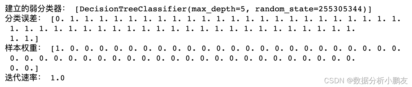
3.4 Adaboost模型训练
abc = AdaBoostClassifier(base_estimator=DecisionTreeClassifier(max_depth=5))
abc.fit(x_train,y_train)

print("建立的弱分类器:",abc.estimators_)
print("分类误差:",abc.estimator_errors_)
print("分类器权重:",abc.estimator_weights_)
print("迭代速率:",abc.learning_rate)
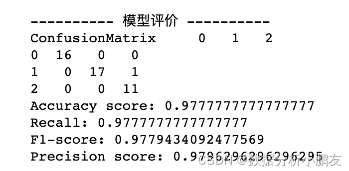
3.5 模型预测与评价
y_pred = abc.predict(x_test)

print("\n---------- 模型评价 ----------")
cm = confusion_matrix(y_test, y_pred)
df_cm = pd.DataFrame(cm)
print("ConfusionMatrix",df_cm)
print('Accuracy score:', accuracy_score(y_test, y_pred))
print('Recall:', recall_score(y_test, y_pred, average='weighted'))
print('F1-score:', f1_score(y_test, y_pred, average='weighted'))
print('Precision score:', precision_score(y_test, y_pred, average='weighted'))
Original: https://blog.csdn.net/small__roc/article/details/124451712
Author: 数据分析小鹏友
Title: Adaboost分类算法原理及代码实例 python
原创文章受到原创版权保护。转载请注明出处:https://www.johngo689.com/661890/
转载文章受原作者版权保护。转载请注明原作者出处!