

《MATLAB语音信号分析与合成(第二版)》:第9章 共振峰的估算方法
- 前言
- 1. 数据与函数路径设置
- 2. MATLAB仿真一:倒谱法对共振峰的估算
- 3. MATLAB仿真二:LPC法对共振峰的估算一
- 4. MATLAB仿真三:LPC法对共振峰的估算二
- 5. MATLAB仿真四:连续语音LPC法共振峰的检测一
- 6. MATLAB仿真五:连续语音LPC法共振峰的检测二
- 7. MATLAB仿真六:基于希尔伯特黄变换HHT的共振峰检测一
- 8. MATLAB仿真七:基于希尔伯特黄变换HHT的共振峰检测二
- 小结
前言
《MATLAB语音信号分析与合成(第二版)》是中科院声学所的大佬宋知用老师数十年经验积累下的呕心之作,对于语音信号处理相关感兴趣的同学,日后希望在语音信号分析、处理与合成相关领域进行一定研究的话,可以以此进行入门。
语音信号处理是数字信号处理的一个重要分支。本书含有许多数字信号处理的方法和 MATLAB函数。 全书共10章。第1-4章介绍语音信号处理的一些基本分析方法和手段,以及相应的MATLAB函数;第5-9章介绍语音信号预处理和特征的提取,包括消除趋势项和基本的减噪方法,以及端点检测、基音的提取和共 振峰的提取,并利用语音信号处理的基本方法,给出了多种提取方法和相应的 MATLAB程序;第10章结合 各种参数的检测介绍了语音信号的合成、语音信号的变速和变调处理,还介绍了时域基音同步叠加( TD PSOLA)的语音合成,并给出了相应的MATLAB程序。附录A中给出了调试复杂程序的方法和思路。 本书可作为从事语音信号处理的本科高年级学生、研究生或科研工程技术人员的辅助读物,也可作为从 事信号处理研究与应用的科研工程技术人员的参考用书。
我的研究生导师的主要方向是语音信号处理。虽然我研究生期间的主要论文是数字图像处理,但所谓的语音和图像是分不开的。虽然我是在老师的研究生主讲的小波变换上划桨,但在后来的导师的语音信号处理课程设计和工程应用中,我也收录了一点语音。他在收官测试中获得小组第一名,辅导老师还特意给他发了300美元的餐费鼓励。
[En]
The main direction of my graduate tutor is related to speech signal processing. Although my major thesis during my postgraduate period is digital image processing, the so-called speech and image are not separated. Although I paddle on the wavelet transform of the teacher’s main graduate lecture, but in the later tutor’s speech signal processing course design and engineering application, I also included a little bit of speech. He won the first place in the group in the closing test, and the tutor specially handed out a meal fund of 300 US dollars to encourage him.
这次拿起语音识别,刚刚从宋先生的书开始,算是自己的点评,主要介绍每一章的源代码,这是该书第九章的七个模拟应用实例,不用说,就开始吧!
[En]
This time to pick up speech recognition, just started with Mr. Song’s book, can be regarded as their own review, mainly to introduce the source code in each chapter, this is the ninth chapter of the book’s seven simulation application examples, not to say much, start!
- 数据与函数路径设置
书中经常会调用的一些函数(自编函数或取自其他应用工具箱中的函数)已集中在basic_tbx工具箱中,在运行本书的程序前请把该工具箱设置(用set path设置)在工作路径下;
当要运行EMD处理时,要把emd工具箱设置在工作路径下;
当要运行主体延伸基音检测时,要把Pitch_ztlib工具箱设置在工作路径下;
当要进行时域基音同步叠加语音合成时,要把psola_lib工具箱设置在工作路径下;
当要应用本书提供的语音数据时,最好把speech_signal设置在工作路径下。
本书的所有函数和程序都在MATLAB R2009a版本下调试通过。(我用的是MATLAB2015b,有些函数已经更新,所以我会进行修改,以便调试通过)
路径设置的方法如下:
打开MATLAB,点击”主页”,找到设置路径

将上述文件夹路径全部添加到MATLAB搜索路径中
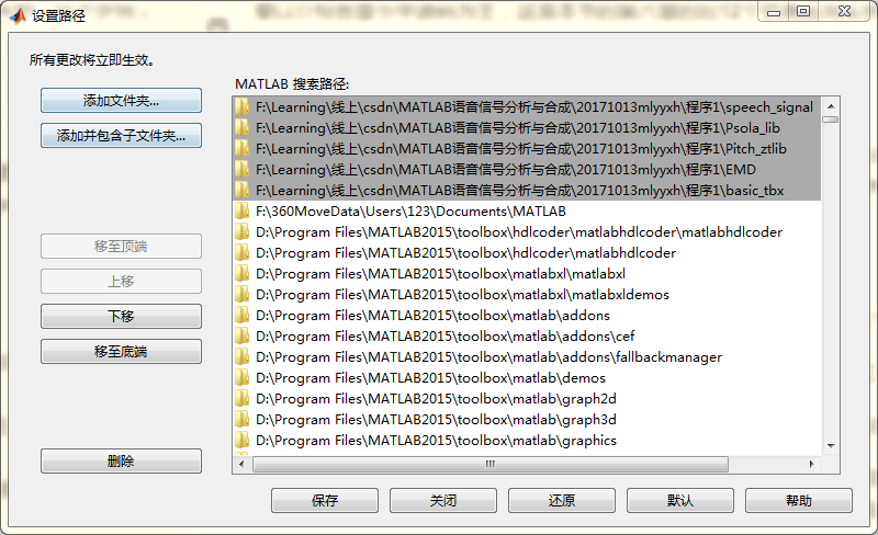
添加、保存和启动仿真。
[En]
Add, save, and start the simulation.
; 2. MATLAB仿真一:倒谱法对共振峰的估算
%
% pr9_2_1
clear all; clc; close all;
waveFile='snn27.wav'; % 设置文件名
% [x, fs, nbits]=wavread(waveFile); % 读入一帧数据
[x, fs]=audioread(waveFile); % 读入一帧数据
u=filter([1 -.99],1,x); % 预加重
wlen=length(u); % 帧长
cepstL=6; % 倒频率上窗函数的宽度
wlen2=wlen/2;
freq=(0:wlen2-1)*fs/wlen; % 计算频域的频率刻度
u2=u.*hamming(wlen); % 信号加窗函数
U=fft(u2); % 按式(9-2-1)计算
U_abs=log(abs(U(1:wlen2))); % 按式(9-2-2)计算
Cepst=ifft(U_abs); % 按式(9-2-3)计算
cepst=zeros(1,wlen2);
cepst(1:cepstL)=Cepst(1:cepstL); % 按式(9-2-5)计算
cepst(end-cepstL+2:end)=Cepst(end-cepstL+2:end);
spect=real(fft(cepst)); % 按式(9-2-6)计算
[Loc,Val]=findpeaks(spect); % 寻找峰值
FRMNT=freq(Loc); % 计算出共振峰频率
% 作图
pos = get(gcf,'Position');
set(gcf,'Position',[pos(1), pos(2)-100,pos(3),(pos(4)-140)]);
plot(freq,U_abs,'k');
hold on; axis([0 4000 -6 2]); grid;
plot(freq,spect,'k','linewidth',2);
xlabel('频率/Hz'); ylabel('幅值/dB');
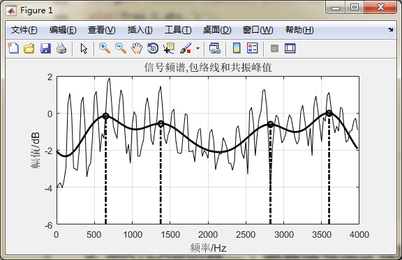
title('信号频谱,包络线和共振峰值')
fprintf('%5.2f %5.2f %5.2f %5.2f\n',FRMNT);
for k=1 : 4
plot(freq(Loc(k)),Val(k),'kO','linewidth',2);
line([freq(Loc(k)) freq(Loc(k))],[-6 Val(k)],'color','k',...
'linestyle','-.','linewidth',2);
end
- MATLAB仿真二:LPC法对共振峰的估算一
%
% pr9_3_1
clear all; clc; close all;
fle='snn27.wav'; % 指定文件名
% [x,fs]=wavread(fle); % 读入一帧语音信号
[x,fs]=audioread(fle); % 读入一帧语音信号
u=filter([1 -.99],1,x); % 预加重
wlen=length(u); % 帧长
p=12; % LPC阶数
a=lpc(u,p); % 求出LPC系数
U=lpcar2pf(a,255); % 由LPC系数求出频谱曲线
freq=(0:256)*fs/512; % 频率刻度
df=fs/512; % 频率分辨率
U_log=10*log10(U); % 功率谱分贝值
subplot 211; plot(u,'k'); % 作图
axis([0 wlen -0.5 0.5]);
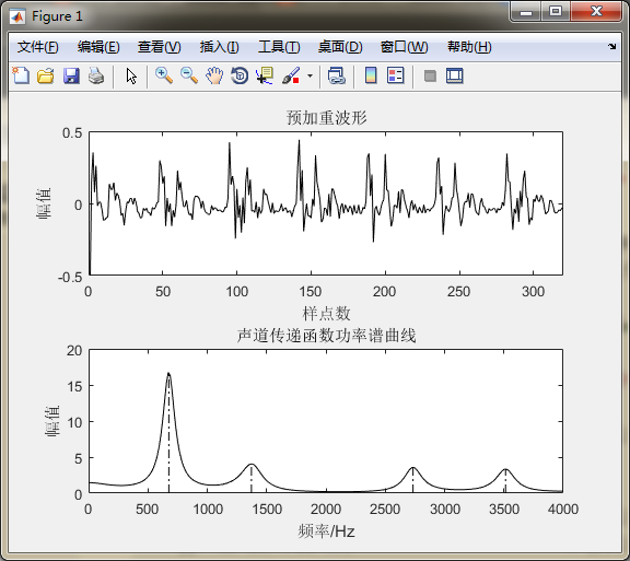
title('预加重波形');
xlabel('样点数'); ylabel('幅值')
subplot 212; plot(freq,U,'k');
title('声道传递函数功率谱曲线');
xlabel('频率/Hz'); ylabel('幅值');
[Loc,Val]=findpeaks(U); % 在U中寻找峰值
ll=length(Loc); % 有几个峰值
for k=1 : ll
m=Loc(k); % 设置m-1,m和m+1
m1=m-1; m2=m+1;
p=Val(k); % 设置P(m-1),P(m)和P(m+1)
p1=U(m1); p2=U(m2);
aa=(p1+p2)/2-p; % 按式(9-3-4)计算
bb=(p2-p1)/2;
cc=p;
dm=-bb/2/aa; % 按式(9-3-6)计算
pp=-bb*bb/4/aa+cc; % 按式(9-3-8)计算
m_new=m+dm;
bf=-sqrt(bb*bb-4*aa*(cc-pp/2))/aa; % 按式(9-3-13)计算
F(k)=(m_new-1)*df; % 按式(9-3-7)计算
Bw(k)=bf*df; % 按式(9-3-14)计算
line([F(k) F(k)],[0 pp],'color','k','linestyle','-.');
end
fprintf('F =%5.2f %5.2f %5.2f %5.2f\n',F)
fprintf('Bw=%5.2f %5.2f %5.2f %5.2f\n',Bw)
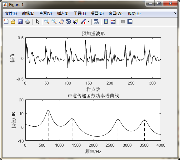
- MATLAB仿真三:LPC法对共振峰的估算二
%
% pr9_3_2
clear all; clc; close all;

fle='snn27.wav';                            % 指定文件名
% [xx,fs]=wavread(fle);                       % 读入一帧语音信号
[xx,fs]=audioread(fle);                       % 读入一帧语音信号
u=filter([1 -.99],1,xx);                    % 预加重
wlen=length(u);                             % 帧长
p=12;                                       % LPC阶数
a=lpc(u,p);                                 % 求出LPC系数
U=lpcar2pf(a,255);                          % 由LPC系数求出功率谱曲线
freq=(0:256)*fs/512;                        % 频率刻度
df=fs/512;                                  % 频率分辨率
U_log=10*log10(U);                          % 功率谱分贝值
subplot 211; plot(u,'k');                   % 作图
axis([0 wlen -0.5 0.5]);
title('预加重波形');
xlabel('样点数'); ylabel('幅值')
subplot 212; plot(freq,U_log,'k');
title('声道传递函数功率谱曲线');
xlabel('频率/Hz'); ylabel('幅值/dB');

n_frmnt=4;                                  % 取四个共振峰
const=fs/(2*pi);                            % 常数
rts=roots(a);                               % 求根
k=1;                                        % 初始化
yf = [];
bandw=[];
for i=1:length(a)-1
    re=real(rts(i));                        % 取根之实部
    im=imag(rts(i));                        % 取根之虚部
    formn=const*atan2(im,re);               % 按(9-3-17)计算共振峰频率
    bw=-2*const*log(abs(rts(i)));           % 按(9-3-18)计算带宽

    if formn>150 & bw <700 & formn<fs/2     % 满足条件方能成共振峰和带宽
        yf(k)=formn;
        bandw(k)=bw;
        k=k+1;
    end
end

[y, ind]=sort(yf);                          % 排序
bw=bandw(ind);
F = [NaN NaN NaN NaN];                      % 初始化
Bw = [NaN NaN NaN NaN];
F(1:min(n_frmnt,length(y))) = y(1:min(n_frmnt,length(y)));   % 输出最多四个
Bw(1:min(n_frmnt,length(y))) = bw(1:min(n_frmnt,length(y))); % 输出最多四个
F0 = F(:);                                  % 按列输出
Bw = Bw(:);
p1=length(F0);                              % 在共振峰处画线
for k=1 : p1
    m=floor(F0(k)/df);
    P(k)=U_log(m+1);
    line([F0(k) F0(k)],[-10 P(k)],'color','k','linestyle','-.');
end
fprintf('F0=%5.2f   %5.2f   %5.2f   %5.2f\n',F0);
fprintf('Bw=%5.2f   %5.2f   %5.2f   %5.2f\n',Bw);
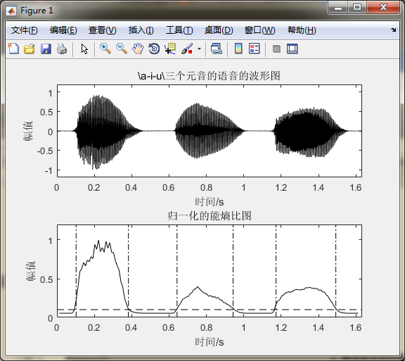
- MATLAB仿真四:连续语音LPC法共振峰的检测一
%
% pr9_4_1
clear all; clc; close all;
filedir=[]; % 设置数据文件的路径
filename='vowels8.wav'; % 设置数据文件的名称
fle=[filedir filename] % 构成路径和文件名的字符串
% [xx,fs]=wavread(fle); % 读入语音文件
[xx,fs]=audioread(fle); % 读入语音文件
x=xx-mean(xx); % 消除 直流分量
x=x/max(abs(x)); % 幅值归一化
y=filter([1 -.99],1,x); % 预加重
wlen=200; % 设置帧长
inc=80; % 设置帧移
xy=enframe(y,wlen,inc)'; % 分帧
fn=size(xy,2); % 求帧数
Nx=length(y); % 数据长度
time=(0:Nx-1)/fs; % 时间刻度
frameTime=frame2time(fn,wlen,inc,fs); % 每帧对应的时间刻度
T1=0.1; % 设置阈值T1和T2的比例常数
miniL=20; % 有话段的最小帧数
p=9; thr1=0.75; % 线性预测阶数和阈值
[voiceseg,vosl,SF,Ef]=pitch_vad1(xy,fn,T1,miniL); % 端点检测
Msf=repmat(SF',1,3); % 把SF扩展为fn×3的数组
formant1=Ext_frmnt(xy,p,thr1,fs); % 提取共振峰信息
Fmap1=Msf.*formant1; % 只取有话段的数据
findex=find(Fmap1==0); % 如果有数值为0 ,设为nan
Fmap=Fmap1;
Fmap(findex)=nan;
nfft=512; % 计算语谱图
d=stftms(y,wlen,nfft,inc);
W2=1+nfft/2;
n2=1:W2;
freq=(n2-1)*fs/nfft;
warning off
% 作图
figure(1) % 画信号的波形图和能熵比图
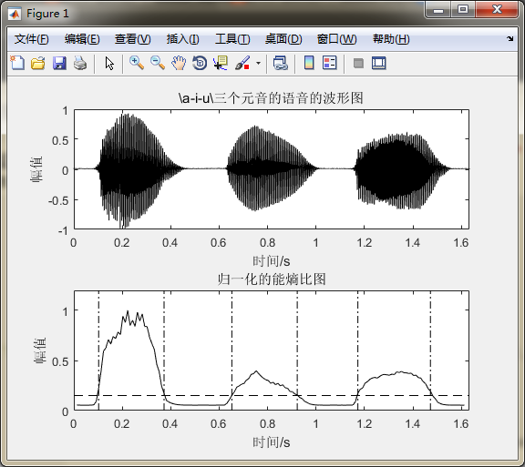
subplot 211; plot(time,x,'k');
title('\a-i-u\三个元音的语音的波形图');
xlabel('时间/s'); ylabel('幅值'); axis([0 max(time) -1.2 1.2]);
subplot 212; plot(frameTime,Ef,'k'); hold on
line([0 max(time)],[T1 T1],'color','k','linestyle','--');
title('归一化的能熵比图'); axis([0 max(time) 0 1.2]);
xlabel('时间/s'); ylabel('幅值')
for k=1 : vosl
in1=voiceseg(k).begin;
in2=voiceseg(k).end;
it1=frameTime(in1);
it2=frameTime(in2);
line([it1 it1],[0 1.2],'color','k','linestyle','-.');
line([it2 it2],[0 1.2],'color','k','linestyle','-.');
end
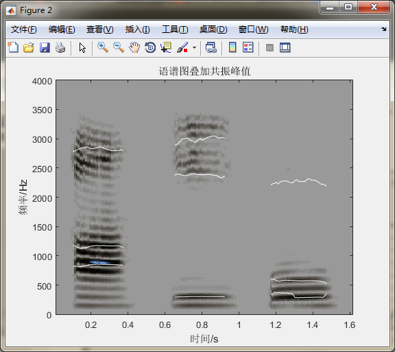
figure(2) % 画语音信号的语谱图
imagesc(frameTime,freq,abs(d(n2,:))); axis xy
m = 64; LightYellow = [0.6 0.6 0.6];
MidRed = [0 0 0]; Black = [0.5 0.7 1];
Colors = [LightYellow; MidRed; Black];
colormap(SpecColorMap(m,Colors)); hold on
plot(frameTime,Fmap,'w'); % 叠加上共振峰频率曲线
title('在语谱图上标出共振峰频率');
xlabel('时间/s'); ylabel('频率/Hz')

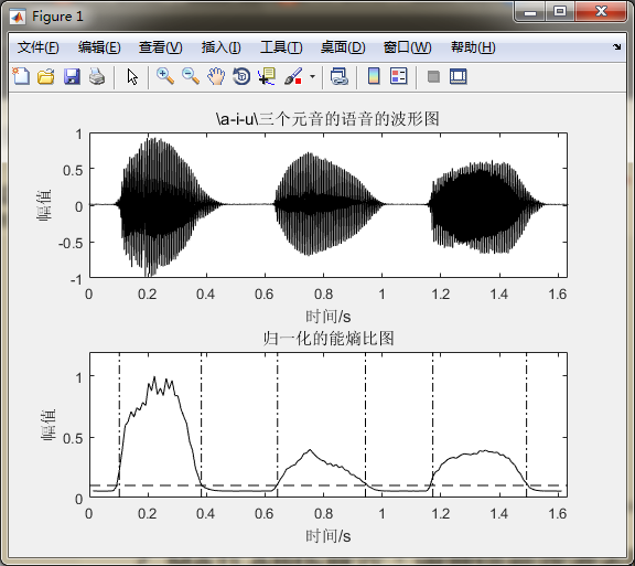
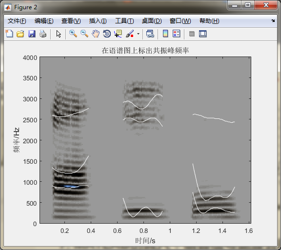
- MATLAB仿真五:连续语音LPC法共振峰的检测二
%
% pr9_4_2
clear all; clc; close all;

filedir=[];                                           % 设置语音文件路径
filename='vowels8.wav';                               % 设置文件名
fle=[filedir filename]
% [x, fs, nbits]=wavread(fle);                          % 读入语音文件
[x, fs]=audioread(fle);                          % 读入语音文件
y=filter([1 -.99],1,x);                               % 预加重
wlen=200;                                             % 设置帧长
inc=80;                                               % 设置帧移
xy=enframe(y,wlen,inc)';                              % 分帧
fn=size(xy,2);                                        % 求帧数
Nx=length(y);                                         % 数据长度
time=(0:Nx-1)/fs;                                     % 时间刻度
frameTime=frame2time(fn,wlen,inc,fs);                 % 每帧对应的时间刻度
T1=0.1;                                               % 判断有话段的能熵比阈值
miniL=10;                                             % 有话段的最小帧数
[voiceseg,vosl,SF,Ef]=pitch_vad1(xy,fn,T1,miniL);     % 端点检测
Msf=repmat(SF',1,3);                                  % 把SF扩展为3×fn的数组
Fsamps = 256;                                         % 设置频域长度
Tsamps= fn;                                           % 设置时域长度
ct = 0;
warning off
numiter = 10;                                         % 循环10次,
iv=2.^(10-10*exp(-linspace(2,10,numiter)/1.9));       % 在0~1024之间计算出10个数
for j=1:numiter
    i=iv(j);
    iy=fix(length(y)/round(i));                       % 计算帧数
    [ft1] = seekfmts1(y,iy,fs,10);                    % 已知帧数提取共振峰
    ct = ct+1;
    ft2(:,:,ct) = interp1(linspace(1,length(y),iy)',...% 把ft1数据内插为Tsamps长
    Fsamps*ft1',linspace(1,length(y),Tsamps)')';
end
ft3 = squeeze(nanmean(permute(ft2,[3 2 1])));         % 重新排列和平均处理
tmap = repmat([1:Tsamps]',1,3);
Fmap=ones(size(tmap))*nan;                            % 初始化
idx = find(~isnan(sum(ft3,2)));                       % 寻找非nan的位置
fmap = ft3(idx,:);                                    % 存放非nan的数据

[b,a] = butter(9,0.1);                                % 设计低通滤波器
fmap1 = round(filtfilt(b,a,fmap));                    % 低通滤波
fmap2 = (fs/2)*(fmap1/256);                           % 恢复到实际频率
Ftmp_map(idx,:)=fmap2;                                % 输出数据

Fmap1=Msf.*Ftmp_map;                                  % 只取有话段的数据
findex=find(Fmap1==0);                                % 如果有数值为0 ,设为nan
Fmap=Fmap1;
Fmap(findex)=nan;

nfft=512;                                             % 计算语谱图
d=stftms(y,wlen,nfft,inc);
W2=1+nfft/2;
n2=1:W2;
freq=(n2-1)*fs/nfft;
% 作图
figure(1)                                             % 画信号的波形图和能熵比图
subplot 211; plot(time,x,'k');
title('\a-i-u\三个元音的语音的波形图');
xlabel('时间/s'); ylabel('幅值'); xlim([0 max(time)]);
subplot 212; plot(frameTime,Ef,'k'); hold on
line([0 max(time)],[T1 T1],'color','k','linestyle','--');
title('归一化的能熵比图'); axis([0 max(time) 0 1.2]);
xlabel('时间/s'); ylabel('幅值')
for k=1 : vosl
    in1=voiceseg(k).begin;
    in2=voiceseg(k).end;
    it1=frameTime(in1);
    it2=frameTime(in2);
    line([it1 it1],[0 1.2],'color','k','linestyle','-.');
    line([it2 it2],[0 1.2],'color','k','linestyle','-.');
end

figure(2)                                             % 画语音信号的语谱图
imagesc(frameTime,freq,abs(d(n2,:)));  axis xy
m = 64; LightYellow = [0.6 0.6 0.6];
MidRed = [0 0 0]; Black = [0.5 0.7 1];
Colors = [LightYellow; MidRed; Black];
colormap(SpecColorMap(m,Colors)); hold on
plot(frameTime,Fmap,'w');                             % 叠加上共振峰频率轨迹
title('在语谱图上标出共振峰频率');
xlabel('时间/s'); ylabel('频率/Hz')
- MATLAB仿真六:基于希尔伯特黄变换HHT的共振峰检测一
%
% pr9_5_1
clear all; clc; close all;
fs=400; % 采样频率
N=400; % 数据长度
n=0:1:N-1;
dt=1/fs;
t=n*dt; % 时间序列
A=0.5; % 相位调制幅值
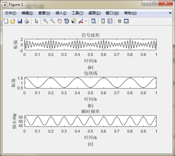
x=(1+0.5*cos(2*pi*5*t)).*cos(2*pi*50*t+A*sin(2*pi*10*t)); % 信号序列
z=hilbert(x'); % 希尔伯特变换
a=abs(z); % 包络线
fnor=instfreq(z); % 瞬时频率
fnor=[fnor(1); fnor; fnor(end)]; % 瞬时频率补齐
% 作图
pos = get(gcf,'Position');
set(gcf,'Position',[pos(1), pos(2)-100,pos(3),pos(4)]);
subplot 311; plot(t,x,'k');
title('信号波形'); ylabel('幅值'); xlabel(['时间/s' 10 '(a)']);
subplot 312; plot(t,a,'k'); ylim([0.4 1.6]);
title('包络线'); ylabel('幅值'); xlabel(['时间/s' 10 '(b)']);
subplot 313; plot(t,fnor*fs,'k'); ylim([43 57]);
title('瞬时频率'); ylabel('频率/Hz'); xlabel(['时间/s' 10 '(c)']);
- MATLAB仿真七:基于希尔伯特黄变换HHT的共振峰检测二
%
% pr9_5_2
clear all; clc; close all;

Formant=[800 1200 3000;                          % 设置元音共振峰参数
    300 2300 3000;
    350 650 2200];
Bwp=[150 200 250];                               % 三个共振峰滤波器的半带宽

filedir=[];                                      % 设置语音文件路径
filename='vowels8.wav';                          % 设置文件名
fle=[filedir filename]                           % 构成语音文件路径和文件名
% [xx, fs, nbits]=wavread(fle);                    % 读入语音
[xx, fs]=audioread(fle);                    % 读入语音
x=filter([1 -.99],1,xx);                         % 预加重
wlen=200;                                        % 帧长
inc=80;                                          % 帧移
y=enframe(x,wlen,inc)';                          % 分帧
fn=size(y,2);                                    % 帧数
Nx=length(x);                                    % 数据长度
time=(0:Nx-1)/fs;                                % 时间刻度
frameTime=frame2time(fn,wlen,inc,fs);            % 每帧的时间刻度
T1=0.15; r2=0.5;                                 % 设置阈值
miniL=10;                                        % 有话段的最小帧数
[voiceseg,vosl,SF,Ef]=pitch_vad1(y,fn,T1,miniL); % 端点检测
FRMNT=ones(3,fn)*nan;                            % 初始化

for m=1 : vosl                                   % 对每一有话段处理
    Frt_cent=Formant(m,:);                       % 取共振峰中心频率
    in1=voiceseg(m).begin;                       % 有话段开始帧号
    in2=voiceseg(m).end;                         % 有话段结束帧号
    ind=in2-in1+1;                               % 有话段长度
    ix1=(in1-1)*inc+1;                           % 有话段在语音中的开始位置
    ix2=(in2-1)*inc+wlen;                        % 有话段在语音中的结束位置
    ixd=ix2-ix1+1;                               % 本有话段长度
    z=x(ix1:ix2);                                % 从语音中取来该有话段
    for kk=1 : 3                                 % 循环3次检测3个共振峰
        fw=Frt_cent(kk);                         % 取来对应的中心频率
        fl=fw-Bwp(kk);                           % 求出滤波器的低截止频率
        if fl<200, fl=200;   end
        fh=fw+Bwp(kk);                           % 求出滤波器的高截止频率
        b=fir1(100,[fl fh]*2/fs);                % 设计带通滤波器
        zz=conv(b,z);                            % 数字滤波
        zz=zz(51:51+ixd-1);                      % 延迟校正
        imp=emd(zz);                             % EMD变换
        impt=hilbert(imp(1,:)');                 % 希尔伯特变换
        fnor=instfreq(impt);                     % 提取瞬时频率
        f0=[fnor(1); fnor; fnor(end)]*fs;        % 长度补齐
        val0=abs(impt);                          % 求模值
        for ii=1 : ind                           % 对每帧计算平均共振峰值
            ixb=(ii-1)*inc+1;                    % 该帧的开始位置
            ixe=ixb+wlen-1;                      % 该帧的结束位置
            u0=f0(ixb:ixe);                      % 取来该帧中的数据
            a0=val0(ixb:ixe);                    % 按式(9-5-17)计算
            a2=sum(a0.*a0);
            v0=sum(u0.*a0.*a0)/a2;
            FRMNT(kk,in1+ii-1)=v0;               % 赋值给FRMNT
        end
    end
end

%nfft=512;                                        % 计算语谱图
%d=stftms(x,wlen,nfft,inc);
%W2=1+nfft/2;
%n2=1:W2;
%freq=(n2-1)*fs/nfft;

% 作图
figure(1)                                        % 画信号的波形图和能熵比图
subplot 211; plot(time,xx,'k');
title('\a-i-u\三个元音的语音的波形图');
xlabel('时间/s'); ylabel('幅值'); xlim([0 max(time)]);
subplot 212; plot(frameTime,Ef,'k'); hold on
line([0 max(time)],[T1 T1],'color','k','linestyle','--');
title('归一化的能熵比图'); axis([0 max(time) 0 1.2]);
xlabel('时间/s'); ylabel('幅值')
for k=1 : vosl
    in1=voiceseg(k).begin;
    in2=voiceseg(k).end;
    it1=frameTime(in1);
    it2=frameTime(in2);
    line([it1 it1],[0 1.2],'color','k','linestyle','-.');
    line([it2 it2],[0 1.2],'color','k','linestyle','-.');
end

figure(2)                                        % 计算语谱图
nfft=512;
d=stftms(x,wlen,nfft,inc);
W2=1+nfft/2;
n2=1:W2;
freq=(n2-1)*fs/nfft;
imagesc(frameTime,freq,abs(d(n2,:)));  axis xy
m = 64; LightYellow = [0.6 0.6 0.6];
MidRed = [0 0 0]; Black = [0.5 0.7 1];
Colors = [LightYellow; MidRed; Black];
colormap(SpecColorMap(m,Colors));
hold on
plot(frameTime,FRMNT(1,:),'w',frameTime,FRMNT(2,:),'w',frameTime,FRMNT(3,:),'w')
title('语谱图叠加共振峰值');
xlabel('时间/s'); ylabel('频率/Hz');
小结
声道可以看作是一个非均匀截面的声管,在发音时起到共振器的作用。当声门处的准周期脉冲激励进入声道时,会产生共振特性,产生一组共振频率,简称共振峰频率或共振峰。共振峰参数包括共振峰频率和带宽(带宽),这是区分不同元音的重要参数。共振峰信息包含在语音谱的包络中,因此提取共振峰参数的关键是对自然语音的谱包络进行估计,认为谱包络的最大值就是共振峰。
[En]
The vocal tract can be regarded as a sound tube with non-uniform cross-section and will act as a resonator when pronouncing. When the quasi-periodic pulse excitation at the glottis enters the sound channel, it will cause resonance characteristics and produce a set of resonance frequencies, which are called formant frequencies or formants for short. Formant parameters include formant frequency and band width (bandwidth), which is an important parameter to distinguish different vowels. Formant information is contained in the envelope of speech spectrum, so the key to formant parameter extraction is to estimate the natural speech spectrum envelope, and it is considered that the maximum of the spectrum envelope is the formant.
与基音提取类似,很难准确估计共振峰,主要表现在以下几个方面:
[En]
Similar to pitch extraction, it is difficult to estimate formants accurately, mainly in the following aspects:
(1) 虚假峰值。在正常情况下,频谱包络中的最大值完全是由共振峰引起的,但有时会出现虚假峰值。
(2) 共振峰合并。当相邻两个共振峰频率靠得很近时难以分辨,而要寻找一种理想的能对共振峰合并进行识别的共振峰提取算法有不少实际的困难。
(3)高音调语音。传统的频谱包络估值方法是利用由谐波峰值提供的样点,而高音调语音(如女声和童声的基音频率较高)的谐波间隔比较宽,因而为频谱包络估值所提供的样点比较少,从而对提取包络带来一定的困难。
如果您对本章内容感兴趣或想全面学习,建议您学习本书第9章的内容。在后期,这些知识点中的一些将在自己理解的基础上进行讨论和补充。欢迎大家一起学习交流。
[En]
If you are interested in the content of this chapter or want to fully learn, it is recommended to study the content of chapter 9 of the book. In the later stage, some of these knowledge points will be discussed and supplemented on the basis of their own understanding. You are welcome to learn and communicate together.
关于宋老师:宋知用——默默传授MATLAB与信号处理知识的老人家
本系列文章列表如下:
《MATLAB语音信号分析与合成(第二版)》:第2章 语音信号的时域、频域特性和短时分析技术
《MATLAB语音信号分析与合成(第二版)》:第3章 语音信号在其他变换域中的分析技术和特性
《MATLAB语音信号分析与合成(第二版)》:第4章 语音信号的线性预测分析
《MATLAB语音信号分析与合成(第二版)》:第5章 带噪语音和预处理
《MATLAB语音信号分析与合成(第二版)》:第6章 语音端点的检测(1)
《MATLAB语音信号分析与合成(第二版)》:第6章 语音端点的检测(2)
《MATLAB语音信号分析与合成(第二版)》:第7章 语音信号的减噪
《MATLAB语音信号分析与合成(第二版)》:第8章 基音周期的估算方法
《MATLAB语音信号分析与合成(第二版)》:第9章 共振峰的估算方法
《MATLAB语音信号分析与合成(第二版)》:第10章 语音信号的合成算法
Original: https://blog.csdn.net/sinat_34897952/article/details/124206404
Author: mozun2020
Title: 《MATLAB语音信号分析与合成(第二版)》:第9章 共振峰的估算方法
原创文章受到原创版权保护。转载请注明出处:https://www.johngo689.com/513122/
转载文章受原作者版权保护。转载请注明原作者出处!