

【基础翻译自:Attention Mechanism For Image Caption Generation in Python
借鉴于:Python中图像标题生成的注意机制实战教程_Together_CZ的博客-CSDN博客】
该文内容主要是针对图像描绘从最基础的baseline:NIC模型开始到引出Attention,并且与Transformer模型进行性能比对,在源内容上进行拓展以及更新。主要针对学期大作业内容进行讲解。
任务定义:
图像描述是一门结合了计算机视觉和自然语言处理两个研究领域的技术。如何高效地输入一幅图像,分析并得到其特征向量,并通过这些特征向量生成通用的句子来正确描述图像是我们的任务。
[En]
Image description is a technology that combines the two research fields of computer vision and natural language processing. How to efficiently input an image, analyze and get its feature vectors, and through these vectors to generate general sentences to correctly describe the image is our task.
现如今较流行的机器学习语言有tensorflow和pytorch两种,在这里主要针对TensorFlow进行编码。
数据集:
该实验基于 Flicker8k 数据集,它是第一个公开的大规模图像和描述匹配的语料集,扩充版本 Flickr30k,其中每一个图像都有五个不同的标题,这些标题描述了图像中所说的实体和事件,我们主要针对 Flicker8k_dateset 和 Flickr8k.token.txt 两个文件进行分析处理,前者放置着图片,后者是每个图片对应的描述语句。通过查询,该数据集图片共有 16182 张,因为存在缺失,图像和描述语句的对应关系只生成了 40455 组,且描述语句最长达到了 33 个单词,反之最短为 2 个单词。最终我们将 dateset 最终设置成了 40000 组进行分析。
数据集的下载可以搜索Flickr8k数据集进行下载。
具体步骤如下:
1.导入所需的库
这里包含了后续所需要的各类models所需要的库,包括VGG16、LSTM等
import string
import numpy as np
import pandas as pd
from numpy import array
from PIL import Image
import pickle
import h5py
import matplotlib.pyplot as plt
import sys, time, os, warnings

warnings.filterwarnings("ignore")
import re

import keras
import tensorflow as tf
import jieba
from tqdm import tqdm
from nltk.translate.bleu_score import sentence_bleu

from keras.preprocessing.sequence import pad_sequences
from keras.utils.np_utils import  to_categorical
from keras.utils.vis_utils import plot_model
from keras.models import Model
from keras.layers import Input
from keras.layers import Dense, BatchNormalization
from keras.layers import LSTM
from keras.layers import Embedding
from keras.layers import Dropout
from keras.layers.merge import add
from keras.callbacks import ModelCheckpoint
from keras.preprocessing.image import load_img, img_to_array
from keras.preprocessing.text import Tokenizer
from keras.applications.vgg16 import VGG16, preprocess_input

from sklearn.utils import shuffle
from sklearn.model_selection import train_test_split
2.数据加载与预处理
Flicker8k_Dataset为图像文档
Flicker8k.token.txt为图像字幕
image_path = "/home/lxx/data/Flicker8k_Dataset"
dir_Flickr_text = "/home/lxx/data/F_t/Flickr8k.token.txt"
jpgs = os.listdir(image_path)

print("Total Images in Dataset = {}".format(len(jpgs)))//查看图像数量
将图像和相对应字幕一一对应:
file = open(dir_Flickr_text, 'r')
text = file.read()
file.close()
#编号图片文字对应
datatxt = []
for line in text.split('\n'):
    col = line.split('\t')
    if len(col) == 1:
        continue
    w = col[0].split("#")
    datatxt.append(w + [col[1].lower()])
print(len(datatxt))
data = pd.DataFrame(datatxt, columns=["filename", "index", "caption"])
data = data.reindex(columns=['index', 'filename', 'caption'])
data = data[data.filename != '2258277193_586949ec62.jpg.1']
uni_filenames = np.unique(data.filename.values)

data.head()
接下来需要对词汇进行处理
针对描述语句,我们的建立所需要的词典,方便后期描述语句的转化。对于文本,我们需要进行处理,比如删除标点符号、单个字符和数字值,并将出去后的文本分割得到总数量。对于词典部分,我们录用使用率前5000 个的单词来构成 tokenizer, 即使用频率较低单词设为
#词汇
vocabulary = []
for txt in data.caption.values:
   vocabulary.extend(txt.split())
print('Vocabulary Size: %d' % len(set(vocabulary)))

​
def remove_punctuation(text_original):#删除标点
    text_no_punctuation = text_original.translate(string.punctuation)
    return (text_no_punctuation)

def remove_single_character(text):#删除单个
    text_len_more_than1 = ""
    for word in text.split():
        if len(word) > 1:
            text_len_more_than1 += " " + word
    return (text_len_more_than1)

def remove_numeric(text):#删除数字
    text_no_numeric = ""
    for word in text.split():
        isalpha = word.isalpha()#判断是否只含有字母
        if isalpha:
            text_no_numeric += " " + word
    return (text_no_numeric)

def text_clean(text_original):
    text = remove_punctuation(text_original)
    text = remove_single_character(text)
    text = remove_numeric(text)
    return (text)

for i, caption in enumerate(data.caption.values):
    newcaption = text_clean(caption)
    data["caption"].iloc[i] = newcaption

clean_vocabulary = []
for txt in data.caption.values:
   clean_vocabulary.extend(txt.split())
print('Clean Vocabulary Size: %d' % len(set(clean_vocabulary)))
对于每个副标题,我们需要添加
[En]
For each subtitle, we need to add
#增加<start>与<end>
PATH = "/home/lxx/data/Flicker8k_Dataset"
all_captions = []
for caption in data["caption"].astype(str):
caption = '<start> ' + caption + ' <end>'
all_captions.append(caption)
print(all_captions[:10])
</end></start></end></start>
之后我们采取前40000个图像进行处理(批处理大小为64,则一共有625批次)
#每个标题的对应文件
all_img_name_vector = []
for annot in data["filename"]:
    full_image_path = PATH +"/"+ annot
    all_img_name_vector.append(full_image_path)

print(all_img_name_vector[:10])

print(f"len(all_img_name_vector) : {len(all_img_name_vector)}")
print(f"len(all_captions) : {len(all_captions)}")

#仅取40000
def data_limiter(num, total_captions, all_img_name_vector):
    train_captions, img_name_vector = shuffle(total_captions, all_img_name_vector, random_state=1)#随机排列
    train_captions = train_captions[:num]
    img_name_vector = img_name_vector[:num]
    return train_captions, img_name_vector

train_captions, img_name_vector = data_limiter(40000, all_captions, all_img_name_vector)
3.模型构建
在这里我们将采用两种结构来定义图像特征提取模型:VGG16与Inception_v3。
这里两个模型都是用来对图像进行分类,在图像描述中,我们需要的是最后的特征值,因此需要模型中删除了softmax层。
这里我们需要注意的是两者之间的区别:
[En]
What we need to note here is the difference between the two:
1) load_picture中VGG16统一为(224,224),而Inception_V3为(299,299)
2)Inception_V3输出模型为(8,8,2048)《=》(64,2048)
VGG16输出模型为(7,7,512)《=》(49,512)
后面会进行介绍原因,例子呈现Inception_v3。
#使用inception_v3定义
def load_image(image_path):
    img = tf.io.read_file(image_path)
    img = tf.image.decode_jpeg(img, channels=3)
    img = tf.image.resize(img, (299, 299))
    img = tf.keras.applications.inception_v3.preprocess_input(img)
    return img, image_path

image_model = tf.keras.applications.InceptionV3(include_top=False, weights='imagenet')
new_input = image_model.input
hidden_layer = image_model.layers[-1].output
image_features_extract_model = tf.keras.Model(new_input, hidden_layer)

image_features_extract_model.summary()
模型结构————inception_v3


模型结构————VGG16

接下来,让我们将每个图片名称映射到要加载图片的函数。
[En]
Next, let’s map each picture name to the function that you want to load the picture.
#映射
encode_train = sorted(set(img_name_vector))
image_dataset = tf.data.Dataset.from_tensor_slices(encode_train)
image_dataset = image_dataset.map(load_image, num_parallel_calls=tf.data.experimental.AUTOTUNE).batch(64)
我们将特征存储在各自的.npy文件中,然后将这些特征通过编码器传递。
#提取特征并将其存储在各自的.npy文件中
for img, path in tqdm(image_dataset):
    batch_features = image_features_extract_model(img)
    batch_features = tf.reshape(batch_features,
                                (batch_features.shape[0], -1, batch_features.shape[3]))

    for bf, p in zip(batch_features, path):
        path_of_feature = p.numpy().decode("utf-8")
        np.save(path_of_feature, bf.numpy())
之后,我们会建立一个词典,根据出现的次数将词汇量设置为5000,并将未放置的单词设置为
[En]
After that, we will set up a dictionary, set the vocabulary to 5000 according to the number of occurrences, and set the unplaced words to
top_k = 5000
tokenizer = tf.keras.preprocessing.text.Tokenizer(num_words=top_k,
oov_token="<unk>",
filters='!"#$%&()*+.,-/:;=?@[\]^_`{|}~ ')#分词器
tokenizer.fit_on_texts(train_captions)#使用一系列文档来生成token词典
train_seqs = tokenizer.texts_to_sequences(train_captions)#将多个文档转换为word下标的向量形式
tokenizer.word_index['<pad>'] = 0## 词_索引 保存所有word对应的编号id 从1开始
tokenizer.index_word[0] = '<pad>'
train_seqs = tokenizer.texts_to_sequences(train_captions)
cap_vector = tf.keras.preprocessing.sequence.pad_sequences(train_seqs, padding='post')</pad></pad></unk>
计算所有字幕的长度,以便后续填充到统一的长度
[En]
Calculate the length of all subtitles to facilitate subsequent filling to a uniform length
def calc_max_length(tensor):
    return max(len(t) for t in tensor)

max_length = calc_max_length(train_seqs)

def calc_min_length(tensor):
    return min(len(t) for t in tensor)

min_length = calc_min_length(train_seqs)

print('Max Length of any caption : Min Length of any caption = ' + str(max_length) + " : " + str(min_length))
划分训练集和验证集,比例分别为80%和20%
[En]
Divide training set and verification set, with a ratio of 80% and 20%
img_name_train, img_name_val, cap_train, cap_val = train_test_split(img_name_vector,cap_vector, test_size=0.2, random_state=0)#使用80-20拆分创建训练和验证集
训练参数定义
这里仍按照Inception_V3进行编写,若想要变成VGG16,按照上述改变输出输出形状即可
定义训练参数:
BATCH_SIZE = 64
BUFFER_SIZE = 1000
embedding_dim = 256
units = 512
vocab_size = len(tokenizer.word_index) + 1
num_steps = len(img_name_train) // BATCH_SIZE
InceptionV3模型的输出形状为(8, 8, 2048)即(64, 2048)
对应attention_features_shape和features_shape
features_shape = 2048
attention_features_shape = 64
加载npy到内存
def map_func(img_name, cap):
    img_tensor = np.load(img_name.decode('utf-8') + '.npy')
    return img_tensor, cap

dataset = tf.data.Dataset.from_tensor_slices((img_name_train, cap_train))
使用dataset的map方法并行调用map_func函数, 将数据集加载到内存中
dataset = dataset.map(lambda item1, item2: tf.numpy_function(map_func, [item1, item2], [tf.float32, tf.int32]),
                      num_parallel_calls=tf.data.experimental.AUTOTUNE)
将数据集成批次的进行打乱
dataset = dataset.shuffle(BUFFER_SIZE).batch(BATCH_SIZE)
根据当前硬件的资源情况,会在模型训练同时预取数据到内存中, 加快训练速度
dataset = dataset.prefetch(buffer_size=tf.data.experimental.AUTOTUNE)
Inception_V3模型结构
class InceptionV3_Encoder(tf.keras.Model):
    # This encoder passes the features through a Fully connected layer
    def __init__(self, embedding_dim):
        super(InceptionV3_Encoder, self).__init__()
        # shape after fc == (batch_size, 49, embedding_dim)
        self.fc = tf.keras.layers.Dense(embedding_dim)#全连接层
        self.dropout = tf.keras.layers.Dropout(0.5, noise_shape=None, seed=None)#防止过拟合

    def call(self, x):
        # x= self.dropout(x)
        x = self.fc(x)
        x = tf.nn.relu(x)#将输入小于0的值幅值为0,输入大于0的值不变
        return x
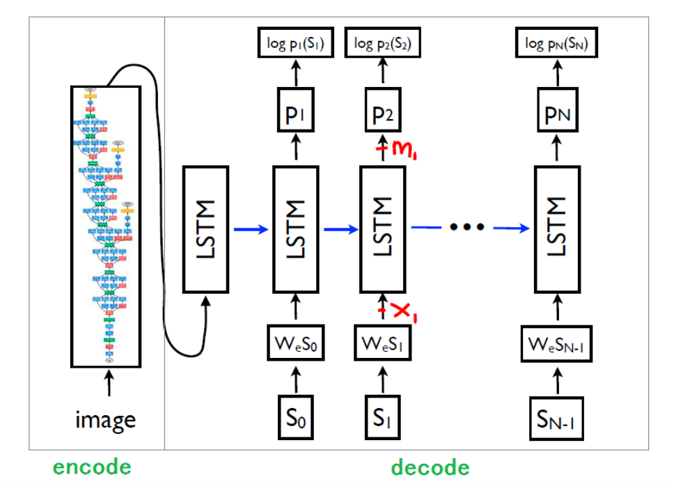
基准系统:NIC实现(无注意力)
该实验的 baseline 主要是基于 Google 提出的 NIC 模型,即 CNN-RNN 模型,利用简单的 CNN 卷积网络作为编辑器,其中用了三个卷积层,卷积核都为 3,步长为1,pooling 层都用MAX 实现简单的提取图像特征功能,而RNN 循环神经网络作为解码器。具体过程是将经过 CNN 卷积层的图像特征作为 RNN 的首个输入值,然后在依次将描述语句分解输入到RNN 中进行训练,训练方式同样采取teacher-forcing方法,具体过程如图 5, 而图 5 的 RNN 采用 LSTM 实现,和 GRU 一样,能很大程度上缓解 RNN 的梯度爆炸问题。
代码如下:
class Rnn_Local_Decoder(tf.keras.Model):
    def __init__(self, embedding_dim, units, vocab_size):
        super(Rnn_Local_Decoder, self).__init__()
        self.units = units
        self.embedding = tf.keras.layers.Embedding(vocab_size, embedding_dim)
        self.gru = tf.keras.layers.GRU( self.units,
                                       return_sequences=True,
                                       return_state=True,
                                       recurrent_initializer='glorot_uniform')

        self.fc1 = tf.keras.layers.Dense(self.units)

        self.dropout = tf.keras.layers.Dropout(0.5, noise_shape=None, seed=None)
        self.batchnormalization = tf.keras.layers.BatchNormalization(axis=-1, momentum=0.99, epsilon=0.001, center=True,
                                                                     scale=True, beta_initializer='zeros',
                                                                     gamma_initializer='ones',
                                                                     moving_mean_initializer='zeros',
                                                                     moving_variance_initializer='ones',
                                                                     beta_regularizer=None, gamma_regularizer=None,
                                                                     beta_constraint=None, gamma_constraint=None)

        self.fc2 = tf.keras.layers.Dense(vocab_size)
        self.fc3 = tf.keras.layers.Dense(embedding_dim)

    def call(self, x, features, hidden,i):

        # 输入通过embedding 层, 得到的输出形状: (batch_size, 1, emb#自己添加到内容
        features=tf.keras.layers.Flatten()(features)
        features=self.dropout(features)
        features=self.fc3(features)
        # features=tf.nn.softmax(features)
        features=tf.expand_dims(features, 1)
        # print(hidden.shape)
        # hidden=self.fc3(hidden)
        hidden=tf.expand_dims(hidden, 1)
        # embdding_dim)== (64, 1, 256)
        x = self.embedding(x)

        # x shape after concatenation == (64, 1,  512)
        # 连接x和注意力结果, 获得新的输出x,形状为: (batch_size, 1, embedding_dim + hidden_size)
        # x = tf.concat([features, x], axis=-1)    # x shape after concatenation == (64, 1,  512)
        # passing the concatenated vector to the GRU
        # print(x)

        if i == 1:
            x = tf.concat([features, hidden], axis=-1)
            output, state = self.gru(x)
        else:
            x = tf.concat([x, hidden], axis=-1)
            output, state = self.gru(x)
        # shape == (batch_size, max_length, hidden_size)

        x = self.fc1(output)
        # x shape == (batch_size * max_length, hidden_size)

        x = tf.reshape(x, (-1, x.shape[2]))

        # Adding Dropout and BatchNorm Layers
        x = self.dropout(x)
        x = self.batchnormalization(x)

        # output shape == (64 * 512)
        x = self.fc2(x)
        # shape : (64 * 8329(vocab))
        return x, state

    def reset_state(self, batch_size):
        return tf.zeros((batch_size, self.units))
使用注意力机制:
#使用Bahdanau注意定义RNN解码器:

class BahdanauAttention(tf.keras.Model):
    def __init__(self, units):
        """初始化三个必要的全连接层"""
        super(BahdanauAttention, self).__init__()
        self.W1 = tf.keras.layers.Dense(units)
        self.W2 = tf.keras.layers.Dense(units)
        self.V = tf.keras.layers.Dense(1)

    def call(self, features, hidden):
"""
        description: 具体计算函数
        :param features: 编码器的输出
        :param hidden: 解码器的隐层输出
        return: 通过注意力机制处理后的结果context_vector和注意力权重attention_weights
"""
        # 为hidden扩展一个维度(batch_size, hidden_size) --> (batch_size, 1, hidden_size)
        hidden_with_time_axis = tf.expand_dims(hidden, 1)

        # 根据公式计算注意力得分, 输出score的形状为: (batch_size, 64, hidden_size)
        score = tf.nn.tanh(self.W1(features) + self.W2(hidden_with_time_axis))

        # 根据公式计算注意力权重, 输出attention_weights形状为: (batch_size, 64, 1)
        attention_weights = tf.nn.softmax(self.V(score), axis=1)

        # 最后根据公式获得注意力机制处理后的结果context_vector
        # context_vector的形状为: (batch_size, hidden_size)
        context_vector = attention_weights * features
        context_vector = tf.reduce_sum(context_vector, axis=1)
        return context_vector, attention_weights

class Rnn_Local_Decoder(tf.keras.Model):
    def __init__(self, embedding_dim, units, vocab_size):
        super(Rnn_Local_Decoder, self).__init__()
        self.units = units
        self.embedding = tf.keras.layers.Embedding(vocab_size, embedding_dim)
        self.gru = tf.keras.layers.GRU( self.units,
                                       return_sequences=True,
                                       return_state=True,
                                       recurrent_initializer='glorot_uniform')

        self.fc1 = tf.keras.layers.Dense(self.units)

        self.dropout = tf.keras.layers.Dropout(0.5, noise_shape=None, seed=None)
        self.batchnormalization = tf.keras.layers.BatchNormalization(axis=-1, momentum=0.99, epsilon=0.001, center=True,
                                                                     scale=True, beta_initializer='zeros',
                                                                     gamma_initializer='ones',
                                                                     moving_mean_initializer='zeros',
                                                                     moving_variance_initializer='ones',
                                                                     beta_regularizer=None, gamma_regularizer=None,
                                                                     beta_constraint=None, gamma_constraint=None)

        self.fc2 = tf.keras.layers.Dense(vocab_size)
        self.fc3 = tf.keras.layers.Dense(embedding_dim)

        self.attention = BahdanauAttention(self.units)

    def call(self, x, features, hidden,i):
        # features shape ==> (64,49,256) ==> Output from ENCODER
        # hidden shape == (batch_size, hidden_size) ==>(64,512)
        # hidden_with_time_axis shape == (batch_size, 1, hidden_size) ==> (64,1,512)

        # hidden_with_time_axis = tf.expand_dims(hidden, 1)

        # score shape == (64, 49, 1)
        # Attention Function
        '''e(ij) = f(s(t-1),h(j))'''
        ''' e(ij) = Vattn(T)*tanh(Uattn * h(j) + Wattn * s(t))'''

        # score = self.Vattn(tf.nn.tanh(self.Uattn(features) + self.Wattn(hidden_with_time_axis)))

        # self.Uattn(features) : (64,49,512)
        # self.Wattn(hidden_with_time_axis) : (64,1,512)
        # tf.nn.tanh(self.Uattn(features) + self.Wattn(hidden_with_time_axis)) : (64,49,512)
        # self.Vattn(tf.nn.tanh(self.Uattn(features) + self.Wattn(hidden_with_time_axis))) : (64,49,1) ==> score

        # you get 1 at the last axis because you are applying score to self.Vattn
        # Then find Probability using Softmax
        '''attention_weights(alpha(ij)) = softmax(e(ij))'''

        # attention_weights = tf.nn.softmax(score, axis=1)

        # attention_weights shape == (64, 49, 1)
        # Give weights to the different pixels in the image
        ''' C(t) = Summation(j=1 to T) (attention_weights * VGG-16 features) '''

        # context_vector = attention_weights * features
        # context_vector = tf.reduce_sum(context_vector, axis=1)
        # features=tf.reduce_sum(features, axis=1)#更改
        # Context Vector(64,256) = AttentionWeights(64,49,1) * features(64,49,256)
        # context_vector shape after sum == (64, 256)
        context_vector, attention_weights = self.attention(features, hidden)

        #自己添加到内容
        features=tf.keras.layers.Flatten()(features)
        features=self.fc3(features)
        features=tf.expand_dims(features, 1)
        # 输入通过embedding 层, 得到的输出形状: (batch_size, 1, embedding_dim)== (64, 1, 256)
        x = self.embedding(x)
        # x shape after concatenation == (64, 1,  512)
        # 连接x和注意力结果, 获得新的输出x,形状为: (batch_size, 1, embedding_dim + hidden_size)
        # x = tf.concat([tf.expand_dims(features, 1), x], axis=-1)    # x shape after concatenation == (64, 1,  512)
        # passing the concatenated vector to the GRU
        # print(x)
        if (i == 1):
            output, state = self.gru(features)
        else:
            output, state = self.gru(x)

        # shape == (batch_size, max_length, hidden_size)

        x = self.fc1(output)
        # x shape == (batch_size * max_length, hidden_size)

        x = tf.reshape(x, (-1, x.shape[2]))

        # Adding Dropout and BatchNorm Layers
        x = self.dropout(x)
        x = self.batchnormalization(x)

        # output shape == (64 * 512)
        x = self.fc2(x)

        # shape : (64 * 8329(vocab))
        return x, state, attention_weights

    def reset_state(self, batch_size):
        return tf.zeros((batch_size, self.units))
编译器和解码器:
encoder 部分我们将完成 GRU 编译和 Bahdanau 注意力机制实现。具体实现步骤是通过根据该算法将图像特征值和隐藏层进行计算得到关联向量和注意力权重,同时连接该步骤输入词向量和注意力,得到一个新的特征向量,并将其输入 GRU 得到所需要的 output,进行多个全连接输出,得到所需要的输出数
encoder = InceptionV3_Encoder(embedding_dim)
decoder = Rnn_Local_Decoder(embedding_dim, units, vocab_size)
损失器和优化器:
encoder = InceptionV3_Encoder(embedding_dim)
decoder = Rnn_Local_Decoder(embedding_dim, units, vocab_size)

#定义损失函数和优化器
optimizer = tf.keras.optimizers.Adam()#优化器 其大概的思想是开始的学习率设置为一个较大的值,然后根据次数的增多,动态的减小学习率,以实现效率和效果的兼得。
loss_object = tf.keras.losses.SparseCategoricalCrossentropy(#交叉熵损失函数
    from_logits=True, reduction='none')

def loss_function(real, pred):
    mask = tf.math.logical_not(tf.math.equal(real, 0))#和0比较返回true和false
    loss_ = loss_object(real, pred)
    mask = tf.cast(mask, dtype=loss_.dtype)
    loss_ *= mask

    return tf.reduce_mean(  loss_)
4.模块训练
在该部分我们选取 Adam 作为优化器以及采用稀疏类别交叉熵损失, 对生成语句和原语句计算 loss,同时我们采用 teacher-forcing 训练方式,即将正确语句的下一个单词强制作为模型的输入进行训练,能够极大的加快模型的收敛速度,令模型训练过程更快更平稳。因为是自定义模型,所以只能通过 save_weights 来保存。最终在获取目标单词构成语句过程中,采用贪婪搜索。
loss_plot = []
@tf.function
def train_step(img_tensor, target):
loss = 0
# 初始化每个批次的隐藏状态
# 因为图片与图片之间的标题不相关
# 初始化解码器的隐含状态张量
hidden = decoder.reset_state(batch_size=target.shape[0])
# 定义解码器的第一个文本描述输入(即起始符<start>对应的张量)
dec_input = tf.expand_dims([tokenizer.word_index['<start>']] * BATCH_SIZE, 1)
# 开启一个用于梯度记录的上下文管理器
with tf.GradientTape() as tape:
# 使用编码器处理输入的图片张量
features = encoder(img_tensor)
# 开始使用解码器循环解码, 解码长度为target.shape[1]即文本描述张量的最大长度
for i in range(1, target.shape[1]):
# passing the features through the decoder
# 使用解码器获得第一个预测值和隐含张量
predictions, hidden, _ = decoder(dec_input, features, hidden)
# 计算该解码过程的损失
loss += loss_function(target[:, i], predictions)
# using teacher forcing
# 接下来这里使用了teacher_forcing来定义下一次解码的输入
dec_input = tf.expand_dims(target[:, i], 1)
# 全部循环解码完成后, 计算句子粒度的平均损失
total_loss = (loss / int(target.shape[1]))
# 获得整个模型训练的参数变量
trainable_variables = encoder.trainable_variables + decoder.trainable_variables
# 使用梯度管理器对象对参数变量求解梯度
gradients = tape.gradient(loss, trainable_variables)
# 根据梯度更新参数
optimizer.apply_gradients(zip(gradients, trainable_variables))
# 返回句子粒度的平均损失
return loss, total_loss
</start></start>
开始训练并且画图
设定训练轮数
EPOCHS = 101

循环轮数训练
for epoch in range(0, EPOCHS):
    # 获得每轮训练的开始时间
    start = time.time()
    # 初始化轮数总损失为0
    total_loss = 0
    # 循环数据集中的每个批次进行训练
    for (batch, (img_tensor, target)) in enumerate(dataset):
        # 调用train_step函数获得批次总损失和批次平均损失
        batch_loss, t_loss = train_step(img_tensor, target)
        # 将批次平均损失相加获得轮数总损失
        total_loss += t_loss
        if batch % 100 == 0:
            print('Epoch {} Batch {} Loss {:.4f}'.format(
                epoch + 1, batch, batch_loss.numpy() / int(target.shape[1])))

    # 绘制轮数平均损失
    loss_plot.append(total_loss / num_steps)
    # 打印轮数, 对应的平均损失
    print('Epoch {} Loss {:.6f}'.format(epoch + 1, total_loss / num_steps))
    # 打印每轮的耗时
    print('Time taken for 1 epoch {} sec\n'.format(time.time() - start))
    if epoch%20==0:
        encoder.save_weights("/home/lxx/data/encoder_ImcepV3_att_%s.h5"%epoch)

        decoder.save_weights("/home/lxx/data/encoder_ImcepV3_att_%s.h5"%epoch)

plt.plot(loss_plot)
plt.xlabel('Epochs')
plt.ylabel('Loss')
plt.title('Loss Plot')
plt.savefig(fname= "VGG16_ImcepV3_100" + ".png")

5.贪婪散发和评估指标
def evaluate(image):
# 初始化用于制图的注意力张量, 为全0张量
attention_plot = np.zeros((max_length, attention_features_shape))
# 初始化隐层张量
hidden = decoder.reset_state(batch_size=1)
# 使用load_image进行图片初始处理, 并扩展一个维度
temp_input = tf.expand_dims(load_image(image)[0], 0)
# 对图片进行特征提取, 并使得形状满足编码器要求
img_tensor_val = image_features_extract_model(temp_input)
img_tensor_val = tf.reshape(img_tensor_val, (img_tensor_val.shape[0], -1, img_tensor_val.shape[3]))
# 使用编码器对图片进行编码
features = encoder(img_tensor_val)
# 初始化解码器的输入张量
dec_input = tf.expand_dims([tokenizer.word_index['<start>']], 0)
# 初始化图片描述的文本结果列表
result = []
# 根据解码器结果生成最终的文本结果
for i in range(max_length):
# 使用解码器获得每次的输出张量
predictions, hidden, attention_weights = decoder(dec_input, features, hidden)
# 根据每次获得的注意力权重填充用于制图的注意力张量
attention_plot[i] = tf.reshape(attention_weights, (-1,)).numpy()
# 从解码器得到的预测概率分布predictions中s随机按概率大小选择索引作为predicted_id
predicted_id = tf.argmax(predictions[0]).numpy()#根据axis取值的不同返回每行或者每列最大值的索引
# 根据数值映射器和predicted_id获得对应单词(文本)并装入结果列表中
result.append(tokenizer.index_word[predicted_id])
# 判断预测字符是否的终止符<end>
if tokenizer.index_word[predicted_id] == '<end>':
return result, attention_plot
# 返回结果列表和用于制图的注意力张量
# 如果不是终止符, 则将本次的结果扩展维度作为下次解码器的输出
dec_input = tf.expand_dims([predicted_id], 0)
# 根据预测结果的真实长度对attention_plot进行切片, 去除多余的为0的部分
attention_plot = attention_plot[:len(result), :]
# 返回结果列表和切片后的注意力张量
return result, attention_plot</end></end></start>
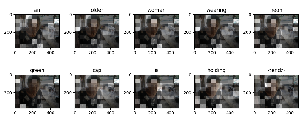
定义一个描述注意力的函数
[En]
Define a function to depict attention
def plot_attention(image, result, attention_plot):
    """注意力可视化函数"""
    # 获得numpy格式的图片表示

    temp_image = np.array(Image.open(image))

    # 创建一个10x10的画板
    fig = plt.figure(figsize=(10, 10))
    # 获得图片描述文本结果长度
    len_result = len(result)
    # 循环结果列表长度
    for l in range(len_result):
        # 将每个结果对应的注意力张量变成8x8的张量
        temp_att = np.resize(attention_plot[l], (8, 8))
        # 创建大小为结果列表长度一半的子图画布
        ax = fig.add_subplot(len_result // 2, len_result // 2, l + 1)
        # 设置子图画布的title
        ax.set_title(result[l])
        # 在子图画布上显示原图片
        img = ax.imshow(temp_image)
        # 在子图画布上显示注意力的灰度块
        ax.imshow(temp_att, cmap='gray', alpha=0.6, extent=img.get_extent())
    # 调整子图位置, 填充整个画布
    plt.tight_layout()
    # 图像显示
    plt.show()
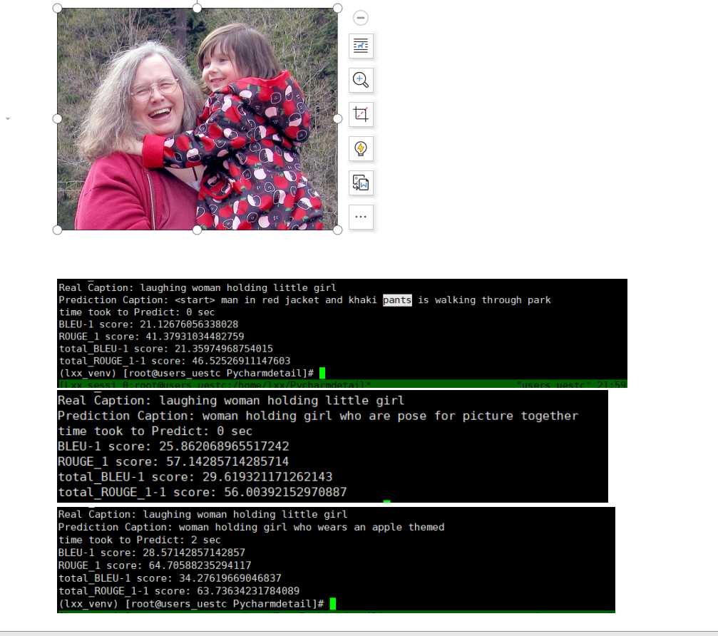
输出效果:
对图像进行测试:
rid = np.random.randint(0, len(img_name_val))
image = img_name_val[rid]
start = time.time()
real_caption = ' '.join([tokenizer.index_word[i] for i in cap_val[rid] if i not in [0]])
result, attention_plot = evaluate(image)

first = real_caption.split(' ', 1)[1]
real_caption = first.rsplit(' ', 1)[0]

remove "<unk>" in result
for i in result:
    if i == "<unk>":
        result.remove(i)

remove <end> from result
result_join = ' '.join(result)
result_final = result_join.rsplit(' ', 1)[0]

real_appn = []
real_appn.append(real_caption.split())
reference = real_appn
candidate = result_final

print('Real Caption:', real_caption)
print('Prediction Caption:', result_final)

plot_attention(image, result, attention_plot)
print(f"time took to Predict: {round(time.time() - start)} sec")

Image.open(img_name_val[rid])</end></unk></unk>
ROUGE_1和BLEU_1测试分数
取100个图进行测试,取平均分(代码与上面有部分重复)
def Rouge_1(target, reference):#terms_reference为参考摘要,terms_model为候选摘要 ***one-gram*** 一元模型
terms_reference= jieba.cut(reference)#默认精准模式
terms_target= jieba.cut(target)
grams_reference = list(terms_reference)
grams_model = list(terms_target)
temp = 0
ngram_all = len(grams_reference)
for x in grams_reference:
if x in grams_model: temp=temp+1
rouge_1=temp/ngram_all
return rouge_1
for z in range(102):
rid = np.random.randint(0, len(img_name_val))
print(rid)
image = img_name_val[rid]
start = time.time()
real_caption = ' '.join([tokenizer.index_word[i] for i in cap_val[rid] if i not in [0]])
result, attention_plot = evaluate(image)
first = real_caption.split(' ', 1)[1]
real_caption = first.rsplit(' ', 1)[0]
# remove "<unk>" in result
for i in result:
if i == "<unk>":
result.remove(i)
if i == "<start>":
result.remove(i)
# remove <end> from result
result_join = ' '.join(result)
# print(result_join)
# print(real_caption)
result_final = result_join.rsplit(' ', 1)[0]#预测
real_appn = []
real_appn.append(real_caption.split())#真实
print('Real Caption:', real_caption)
print('Prediction Caption:', result_final)
# plot_attention(image, result, attention_plot)
# print(f"time took to Predict: {round(time.time() - start)} sec")
total_score=0
total_roughscore=0
score = sentence_bleu(real_caption, result_join, weights=(1, 0, 0, 0))
total_score+=score
total_roughscore+=Rouge_1(real_caption, result_join)
# print(f"BLEU-1 score: {score * 100}")
# print(f"ROUGE_1 score: {Rouge_1(real_caption, result_join) * 100}")
if z==100:
print(f"total_BLEU-1 score: {total_score}")
print(f"total_ROUGE_1 score: {total_roughscore }")
</end></start></unk></unk>
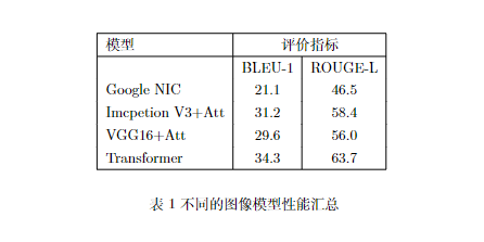
受时间限制,我们针对四个模型都采取在EPOCH=60的条件下进行比对,且针对100幅一样的图进行模型预测。我们可以清楚的发现模型关于BLEU和ROUGE的评分标准从小到大分别是NIC、VGG16+Att、Imception V3+Att、Transformer。我们可以看出Imception V3模型是优于VGG16的,在模型部分可以清楚的看出层数也远远高于它,而Transformer作为最近流行的模型,无论是在训练速度还是评分结果上面都好于其他模型。
未解决的地方:因为这个模型是自己设立的,所以属于subclass,在每次load的时候,我们需要给它赋初始值,他才能正常进行加载模型,在这里我尝试了很多方法,都无法实现这个赋值步骤,只能通过训练一轮并且break来实现初步的赋值,来达到加载功能。
至此,图像描述任务结束了!
[En]
At this point, the image description task is over!
Original: https://blog.csdn.net/weixin_43631804/article/details/123069630
Author: “林仔
Title: 基于tensorflow实现图像描述
原创文章受到原创版权保护。转载请注明出处:https://www.johngo689.com/509480/
转载文章受原作者版权保护。转载请注明原作者出处!