

版本说明
tensorflow 1.8.0
python 3.6.2
conda 3.10.5
h5py 2.10.0
keras 2.1.6
numpy 1.19.3 !!!1.19.4可能会报错!
pandas 0.25.3
- 导入tensorflow库
import math
import numpy as np
import h5py
import matplotlib.pyplot as plt
import tensorflow as tf
from tensorflow.python.framework import ops
from tf_utils import load_dataset, random_mini_batches, convert_to_one_hot, predict

%matplotlib inline
np.random.seed(1)

y_hat = tf.constant(36, name='y_hat')            # Define y_hat constant. Set to 36.

y = tf.constant(39, name='y')                    # Define y. Set to 39

loss = tf.Variable((y - y_hat)**2, name='loss')  # Create a variable for the loss

init = tf.global_variables_initializer()         # When init is run later (session.run(init)),
                                                 # the loss variable will be initialized and ready to be computed
with tf.Session() as session:                    # Create a session and print the output
    session.run(init)                            # Initializes the variables
    print(session.run(loss))                     # Prints the loss
输出 9
在 TensorFlow 中编写和运行程序以下步骤:(大意)
1.创建的张量(变量)。
2.所创建张量之间的操作。
3.初始化张量。
4.创建一个会话。
5.运行会话。
a = tf.constant(2)
b = tf.constant(10)
c = tf.multiply(a,b)
print(c)

sess = tf.Session()
print(sess.run(c))
输出:20
接下来,学习占位符的概念。占位符是一个对象,您只能在定义以后指定其值。要为占位符指定值,您可以使用”字典”(feed_dict 变量)传入值。下面,我们为 x 创建了一个占位符,并在稍后运行会话时传入一个数字。
Change the value of x in the feed_dict

x = tf.placeholder(tf.int64, name = 'x')
print(sess.run(2 * x, feed_dict = {x: 3}))
sess.close()
输出:6
1.1 线性回归
Y = WX + b W,X 随机矩阵 b随机向量
GRADED FUNCTION: linear_function

def linear_function():
"""
    Implements a linear function:
            Initializes W to be a random tensor of shape (4,3)
            Initializes X to be a random tensor of shape (3,1)
            Initializes b to be a random tensor of shape (4,1)
    Returns:
    result -- runs the session for Y = WX + b
"""

    np.random.seed(1)

    ### START CODE HERE ### (4 lines of code)
    X = np.random.randn(3,1)
    W = np.random.randn(4,3)
    b = np.random.randn(4,1)
    Y = tf.add(tf.matmul(W,X),b)
    ### END CODE HERE ###

    # Create the session using tf.Session() and run it with sess.run(...) on the variable you want to calculate

    ### START CODE HERE ###
    sess = tf.Session()
    result = sess.run(Y)

    ### END CODE HERE ###

    # close the session
    sess.close()

    return result

print( "result = " + str(linear_function()))
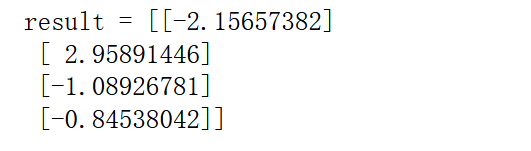
注:X,W,b的初始化顺序不同可能会产生不同结果。
1.2 计算sigmoid
GRADED FUNCTION: sigmoid
def sigmoid(z):
"""
Computes the sigmoid of z
Arguments:
z -- input value, scalar or vector
Returns:
results -- the sigmoid of z
"""
### START CODE HERE ### ( approx. 4 lines of code)
# Create a placeholder for x. Name it 'x'.
x = tf.placeholder(tf.float32, name = "x")
# compute sigmoid(x)
Y = tf.sigmoid(x)
# Create a session, and run it. Please use the method 2 explained above.
# You should use a feed_dict to pass z's value to x. # Run session and call the output "result"
sess = tf.Session()
# Run the variables initialization (if needed), run the operations
result = sess.run(Y, feed_dict = {x:z})
sess.close() # Close the session
### END CODE HERE ###
return result
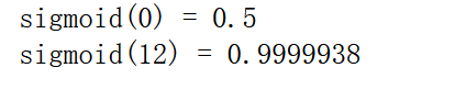
print ("sigmoid(0) = " + str(sigmoid(0)))
print ("sigmoid(12) = " + str(sigmoid(12)))
总结:
1.创建占位符。
2.指定与您要计算的操作相对应的计算图。
3.创建会话。
4.运行会话,必要时使用字典来指定占位符变量的值。
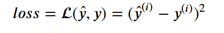
1.3 计算损失函数

GRADED FUNCTION: cost
def cost(logits, labels):
"""
Computes the cost using the sigmoid cross entropy
Arguments:
logits -- vector containing z, output of the last linear unit (before the final sigmoid activation)
labels -- vector of labels y (1 or 0)
Note: What we've been calling "z" and "y" in this class are respectively called "logits" and "labels"
in the TensorFlow documentation. So logits will feed into z, and labels into y.
Returns:
cost -- runs the session of the cost (formula (2))
"""
### START CODE HERE ###
# Create the placeholders for "logits" (z) and "labels" (y) (approx. 2 lines)
z = tf.placeholder(tf.float32, name = "z")
y = tf.placeholder(tf.float32, name = "y")
# Use the loss function (approx. 1 line)
p = tf.nn.sigmoid_cross_entropy_with_logits(logits = z, labels = y)
# Create a session (approx. 1 line). See method 1 above.
sess = tf.Session()
# Run the session (approx. 1 line).
cost = sess.run(p, feed_dict = {z:logits,y:labels})
### END CODE HERE ###
# close the session
sess.close()
# Close the session (approx. 1 line). See method 1 above.
### END CODE HERE ###
return cost
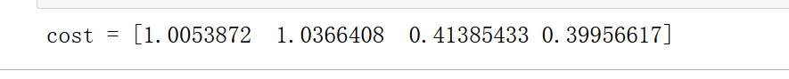
logits = sigmoid(np.array([0.2,0.4,0.7,0.9]))
cost = cost(logits, np.array([0,0,1,1]))
print ("cost = " + str(cost))
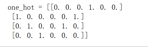
1.4 one-hot编码
GRADED FUNCTION: one_hot_matrix

def one_hot_matrix(labels, C):
"""
    Creates a matrix where the i-th row corresponds to the ith class number and the jth column
                     corresponds to the jth training example. So if example j had a label i. Then entry (i,j)
                     will be 1.

    Arguments:
    labels -- vector containing the labels
    C -- number of classes, the depth of the one hot dimension

    Returns:
    one_hot -- one hot matrix
"""

    ### START CODE HERE ###

    # Create a tf.constant equal to C (depth), name it 'C'. (approx. 1 line)
    C = tf.constant(C ,name="C")

    # Use tf.one_hot, be careful with the axis (approx. 1 line)
    one_hot_matrix = tf.one_hot(indices=labels, depth=C, axis=0)

    # Create the session (approx. 1 line)
    sess = tf.Session()

    # Run the session (approx. 1 line)
    one_hot = sess.run(one_hot_matrix)

    # Close the session (approx. 1 line). See method 1 above.

    sess.close()

    ### END CODE HERE ###

    return one_hot

labels = np.array([1,2,3,0,2,1])
one_hot = one_hot_matrix(labels, C = 4)
print ("one_hot = " + str(one_hot))
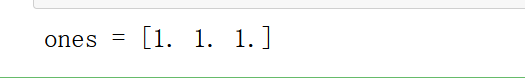
1.5 初始化
GRADED FUNCTION: ones

def ones(shape):
"""
    Creates an array of ones of dimension shape

    Arguments:
    shape -- shape of the array you want to create

    Returns:
    ones -- array containing only ones
"""

    ### START CODE HERE ###

    # Create "ones" tensor using tf.ones(...). (approx. 1 line)
    one = tf.ones(shape)

    # Create the session (approx. 1 line)
    sess = tf.Session()

    # Run the session to compute 'ones' (approx. 1 line)
    ones = sess.run(one)

    # Close the session (approx. 1 line). See method 1 above.

    sess.close()
    ### END CODE HERE ###
    return ones

print ("ones = " + str(ones([3])))
输出:
2.在 tensorflow 中构建你的第一个神经网络
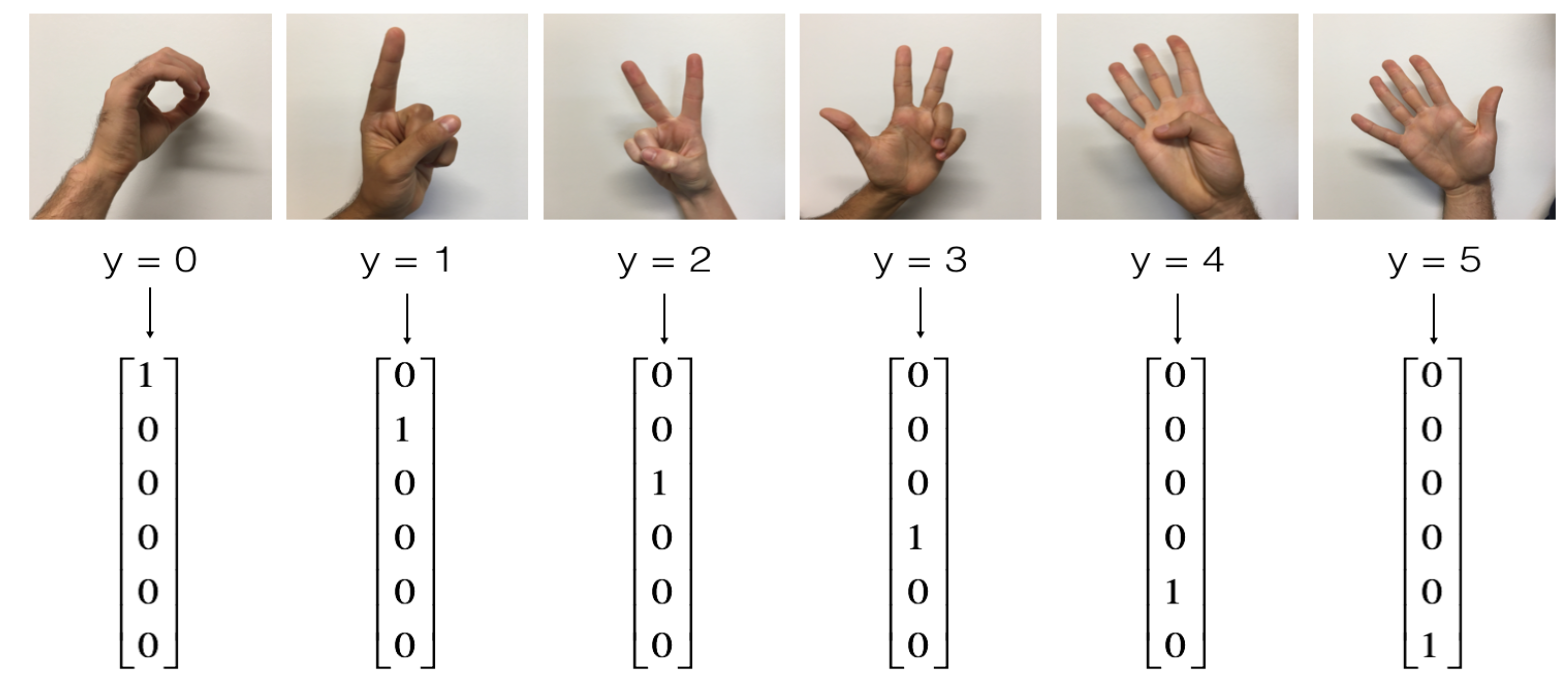
2.0 问题陈述
现在你的工作是建立一个算法来促进语言障碍患者和不懂手语的人之间的交流。
[En]
Now your job is to build an algorithm to facilitate communication between people with language disorders and people who don’t understand sign language.
训练集:1080 张图片(64 x 64 像素)的符号表示从 0 到 5 的数字(每个数字 180 张图片)。
测试集:120 张图片(64 x 64 像素)的符号表示从 0 到 5 的数字(每个数字 20 张图片)。
加载数据集:
Loading the dataset
X_train_orig, Y_train_orig, X_test_orig, Y_test_orig, classes = load_dataset()
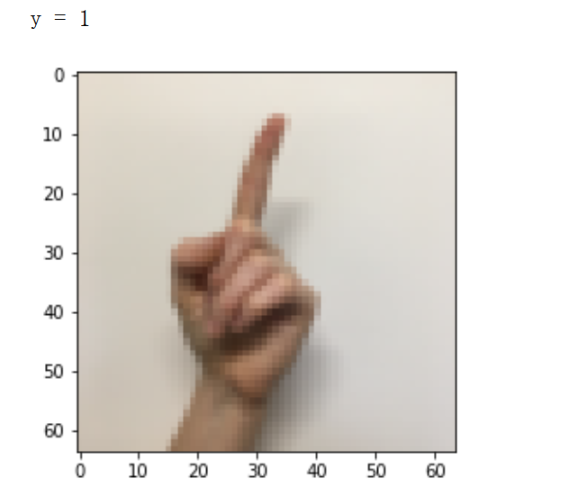
Example of a picture
index = 70
plt.imshow(X_train_orig[index])
print ("y = " + str(np.squeeze(Y_train_orig[:, index])))
数据预处理:
Flatten the training and test images
X_train_flatten = X_train_orig.reshape(X_train_orig.shape[0], -1).T
X_test_flatten = X_test_orig.reshape(X_test_orig.shape[0], -1).T
Normalize image vectors
X_train = X_train_flatten/255.
X_test = X_test_flatten/255.
Convert training and test labels to one hot matrices
Y_train = convert_to_one_hot(Y_train_orig, 6)
Y_test = convert_to_one_hot(Y_test_orig, 6)
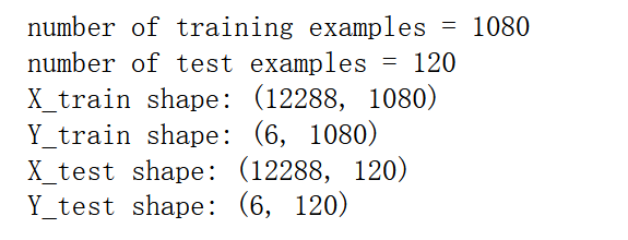
print ("number of training examples = " + str(X_train.shape[1]))
print ("number of test examples = " + str(X_test.shape[1]))
print ("X_train shape: " + str(X_train.shape))
print ("Y_train shape: " + str(Y_train.shape))
print ("X_test shape: " + str(X_test.shape))
print ("Y_test shape: " + str(Y_test.shape))
您的目标是构建一种能够高精度识别标志的算法。为此,您将构建一个 tensorflow 模型,该模型与您之前在 numpy 中构建的用于猫识别的模型几乎相同(但现在使用的是 softmax 输出)。这是一个将您的 numpy 实现与 tensorflow 进行比较的好机会。
模型为 LINEAR -> RELU -> LINEAR -> RELU -> LINEAR -> SOFTMAX。 SIGMOID 输出层已转换为 SOFTMAX。 SOFTMAX 层将 SIGMOID 推广到有两个以上的类情况。
2.1 创建占位符
GRADED FUNCTION: create_placeholders

def create_placeholders(n_x, n_y):
"""
    Creates the placeholders for the tensorflow session.

    Arguments:
    n_x -- scalar, size of an image vector (num_px * num_px = 64 * 64 * 3 = 12288)
    n_y -- scalar, number of classes (from 0 to 5, so -> 6)

    Returns:
    X -- placeholder for the data input, of shape [n_x, None] and dtype "float"
    Y -- placeholder for the input labels, of shape [n_y, None] and dtype "float"

    Tips:
    - You will use None because it let's us be flexible on the number of examples you will for the placeholders.

      In fact, the number of examples during test/train is different.

"""

    ### START CODE HERE ### (approx. 2 lines)
    X = tf.placeholder(tf.float32, [n_x,None],name = "X")
    Y = tf.placeholder(tf.float32, [n_y,None],name = "Y")
    ### END CODE HERE ###

    return X, Y

X, Y = create_placeholders(12288, 6)
print ("X = " + str(X))
print ("Y = " + str(Y))

2.2 初始化参数
GRADED FUNCTION: initialize_parameters
def initialize_parameters():
"""
各个参数的维度如下:
W1 : [25, 12288]
b1 : [25, 1]
W2 : [12, 25]
b2 : [12, 1]
W3 : [6, 12]
b3 : [6, 1]
返回:
parameters - 包含了W和b的字典
"""
tf.set_random_seed(1) #指定随机种子
W1 = tf.get_variable("W1",[25,12288],initializer=tf.contrib.layers.xavier_initializer(seed=1))
b1 = tf.get_variable("b1",[25,1],initializer=tf.zeros_initializer())
W2 = tf.get_variable("W2", [12, 25], initializer = tf.contrib.layers.xavier_initializer(seed=1))
b2 = tf.get_variable("b2", [12, 1], initializer = tf.zeros_initializer())
W3 = tf.get_variable("W3", [6, 12], initializer = tf.contrib.layers.xavier_initializer(seed=1))
b3 = tf.get_variable("b3", [6, 1], initializer = tf.zeros_initializer())
parameters = {"W1": W1,
"b1": b1,
"W2": W2,
"b2": b2,
"W3": W3,
"b3": b3}
return parameters
tf.reset_default_graph()
with tf.Session() as sess:
parameters = initialize_parameters()
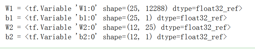
print("W1 = " + str(parameters["W1"]))
print("b1 = " + str(parameters["b1"]))
print("W2 = " + str(parameters["W2"]))
print("b2 = " + str(parameters["b2"]))
输出:
2.3 前向传播过程
GRADED FUNCTION: forward_propagation

def forward_propagation(X, parameters):
"""
    Implements the forward propagation for the model: LINEAR -> RELU -> LINEAR -> RELU -> LINEAR -> SOFTMAX

    Arguments:
    X -- input dataset placeholder, of shape (input size, number of examples)
    parameters -- python dictionary containing your parameters "W1", "b1", "W2", "b2", "W3", "b3"
                  the shapes are given in initialize_parameters

    Returns:
    Z3 -- the output of the last LINEAR unit
"""

    # Retrieve the parameters from the dictionary "parameters"
    W1 = parameters['W1']
    b1 = parameters['b1']
    W2 = parameters['W2']
    b2 = parameters['b2']
    W3 = parameters['W3']
    b3 = parameters['b3']

    ### START CODE HERE ### (approx. 5 lines)              # Numpy Equivalents:
    Z1 = tf.add(tf.matmul(W1,X),b1)
    A1 = tf.nn.relu(Z1)
    Z2 = tf.add(tf.matmul(W2,A1),b2)
    A2 = tf.nn.relu(Z2)
    Z3 = tf.add(tf.matmul(W3,A2),b3)

    ### END CODE HERE ###

    return Z3

tf.reset_default_graph()

with tf.Session() as sess:
    X, Y = create_placeholders(12288, 6)
    parameters = initialize_parameters()
    Z3 = forward_propagation(X, parameters)
    print("Z3 = " + str(Z3))
输出:

2.4 计算损失函数
GRADED FUNCTION: compute_cost

def compute_cost(Z3, Y):
"""
    Computes the cost

    Arguments:
    Z3 -- output of forward propagation (output of the last LINEAR unit), of shape (6, number of examples)
    Y -- "true" labels vector placeholder, same shape as Z3

    Returns:
    cost - Tensor of the cost function
"""

    # to fit the tensorflow requirement for tf.nn.softmax_cross_entropy_with_logits(...,...)
    logits = tf.transpose(Z3)
    labels = tf.transpose(Y)

    ### START CODE HERE ### (1 line of code)
    cost = tf.reduce_mean(tf.nn.softmax_cross_entropy_with_logits(logits = logits, labels = labels))
    ### END CODE HERE ###

    return cost

tf.reset_default_graph()

with tf.Session() as sess:
    X, Y = create_placeholders(12288, 6)
    parameters = initialize_parameters()
    Z3 = forward_propagation(X, parameters)
    cost = compute_cost(Z3, Y)
    print("cost = " + str(cost))
输出:
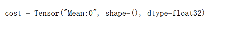
注:出现的warning好像是版本问题,忽略即可~
2.5 反向过程与参数更新
所有反向传播和参数更新都在一行代码中处理。将此行添加到模型中非常容易。
[En]
All backpropagation and parameter updates are handled in one line of code. It is very easy to add this line to the model.
例如,对于渐变下降,优化器可以编写:
[En]
For example, for a gradient drop, the optimizer can write:
optimizer = tf.train.GradientDescentOptimizer(learning_rate = learning_rate).minimize(cost)
要进行优化,您需要执行以下操作:
[En]
To optimize, you will do the following:
_ , c = sess.run([optimizer, cost], feed_dict={X: minibatch_X, Y: minibatch_Y})
2.6 创建模型
def model(X_train, Y_train, X_test, Y_test, learning_rate = 0.005,
num_epochs = 1500, minibatch_size = 64, print_cost = True):
"""
Implements a three-layer tensorflow neural network: LINEAR->RELU->LINEAR->RELU->LINEAR->SOFTMAX.
Arguments:
X_train -- training set, of shape (input size = 12288, number of training examples = 1080)
Y_train -- test set, of shape (output size = 6, number of training examples = 1080)
X_test -- training set, of shape (input size = 12288, number of training examples = 120)
Y_test -- test set, of shape (output size = 6, number of test examples = 120)
learning_rate -- learning rate of the optimization
num_epochs -- number of epochs of the optimization loop
minibatch_size -- size of a minibatch
print_cost -- True to print the cost every 100 epochs
Returns:
parameters -- parameters learnt by the model. They can then be used to predict.
"""
ops.reset_default_graph() # to be able to rerun the model without overwriting tf variables
tf.set_random_seed(1) # to keep consistent results
seed = 3 # to keep consistent results
(n_x, m) = X_train.shape # (n_x: input size, m : number of examples in the train set)
n_y = Y_train.shape[0] # n_y : output size
costs = [] # To keep track of the cost
# Create Placeholders of shape (n_x, n_y)
### START CODE HERE ### (1 line)
X,Y = create_placeholders(n_x, n_y)
### END CODE HERE ###
# Initialize parameters
### START CODE HERE ### (1 line)
parameters = initialize_parameters()
### END CODE HERE ###
# Forward propagation: Build the forward propagation in the tensorflow graph
### START CODE HERE ### (1 line)
Z3 = forward_propagation(X, parameters)
### END CODE HERE ###
# Cost function: Add cost function to tensorflow graph
### START CODE HERE ### (1 line)
cost = compute_cost(Z3, Y)
### END CODE HERE ###
# Backpropagation: Define the tensorflow optimizer. Use an AdamOptimizer.
### START CODE HERE ### (1 line)
optimizer = tf.train.GradientDescentOptimizer(learning_rate = learning_rate).minimize(cost)
### END CODE HERE ###
# Initialize all the variables
init = tf.global_variables_initializer()
# Start the session to compute the tensorflow graph
with tf.Session() as sess:
# Run the initialization
sess.run(init)
# Do the training loop
for epoch in range(num_epochs):
epoch_cost = 0. # Defines a cost related to an epoch
num_minibatches = int(m / minibatch_size) # number of minibatches of size minibatch_size in the train set
seed = seed + 1
minibatches = random_mini_batches(X_train, Y_train, minibatch_size, seed)
for minibatch in minibatches:
# Select a minibatch
(minibatch_X, minibatch_Y) = minibatch
# IMPORTANT: The line that runs the graph on a minibatch.
# Run the session to execute the "optimizer" and the "cost", the feedict should contain a minibatch for (X,Y).
### START CODE HERE ### (1 line)
_,minibatch_cost = sess.run([optimizer,cost],feed_dict={X:minibatch_X,Y:minibatch_Y})
### END CODE HERE ###
epoch_cost += minibatch_cost / num_minibatches
# Print the cost every epoch
if print_cost == True and epoch % 100 == 0:
print ("Cost after epoch %i: %f" % (epoch, epoch_cost))
if print_cost == True and epoch % 5 == 0:
costs.append(epoch_cost)
if epoch%5==0:
costs.append(epoch_cost)
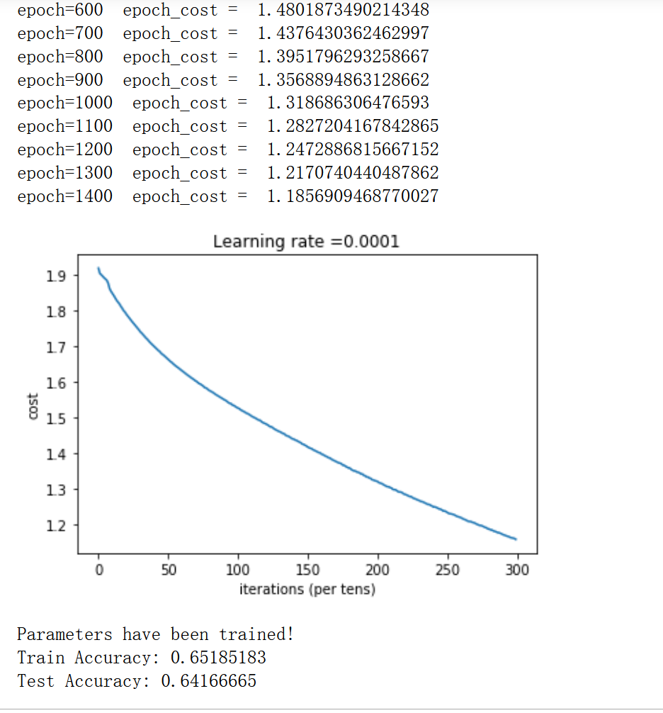
if print_cost and epoch%100==0:
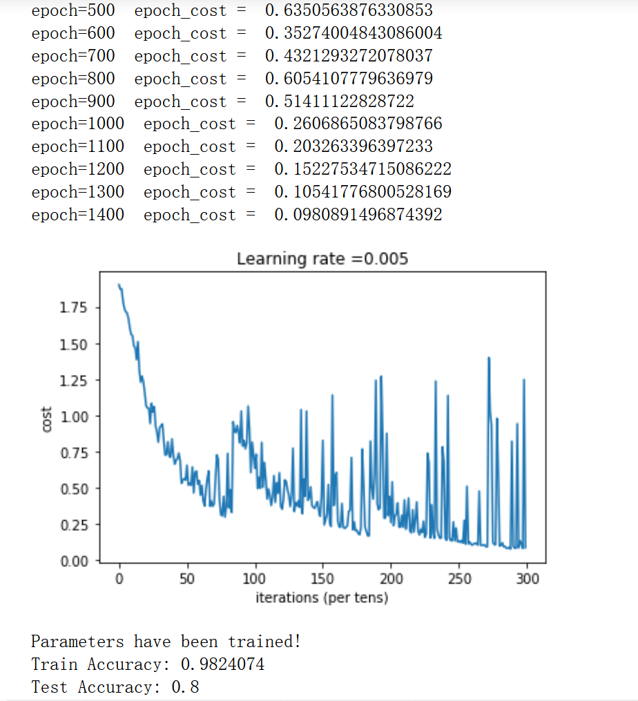
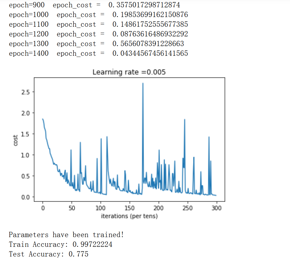
print("epoch="+str(epoch)+" epoch_cost = "+str(epoch_cost))
# plot the cost
plt.plot(np.squeeze(costs))
plt.ylabel('cost')
plt.xlabel('iterations (per tens)')
plt.title("Learning rate =" + str(learning_rate))
plt.show()
# lets save the parameters in a variable
parameters = sess.run(parameters)
print ("Parameters have been trained!")
# Calculate the correct predictions
correct_prediction = tf.equal(tf.argmax(Z3), tf.argmax(Y))
# Calculate accuracy on the test set
accuracy = tf.reduce_mean(tf.cast(correct_prediction, "float"))
print ("Train Accuracy:", accuracy.eval({X: X_train, Y: Y_train}))
print ("Test Accuracy:", accuracy.eval({X: X_test, Y: Y_test}))
return parameters
parameters = model(X_train, Y_train, X_test, Y_test)
注:我调参过程中发现batch_size=64,lr=0.001会得到较好的效果
batch_size = 64 lr = 0.005
batch_size = 64 lr = 0.0001
batch_size = 64 lr = 0.001
batch_size = 64 lr = 0.005
batch_size = 32 lr = 0.005
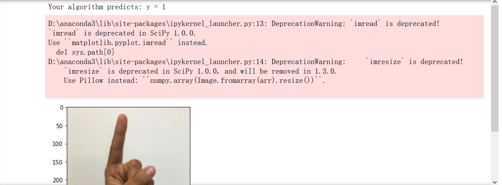
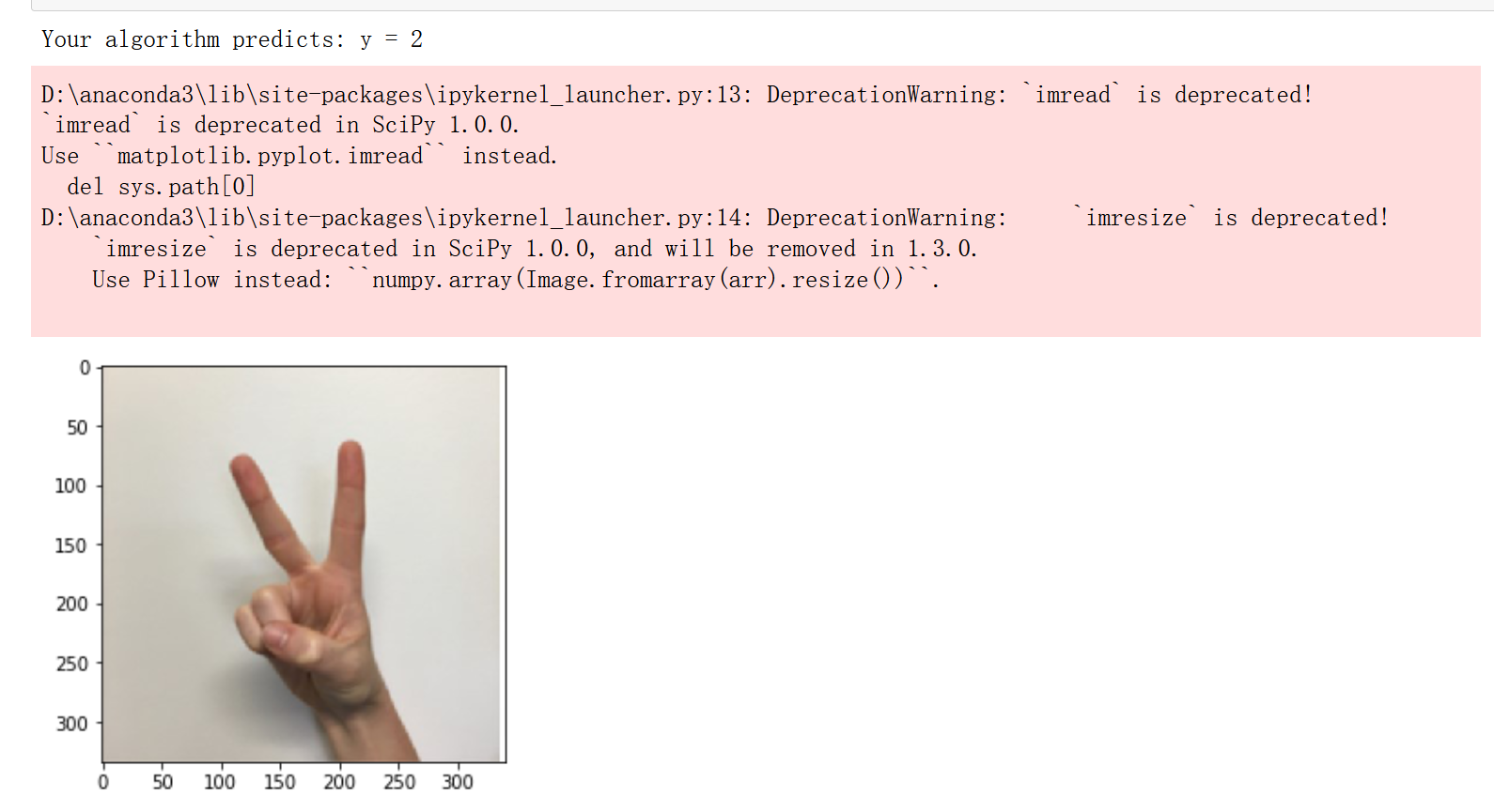
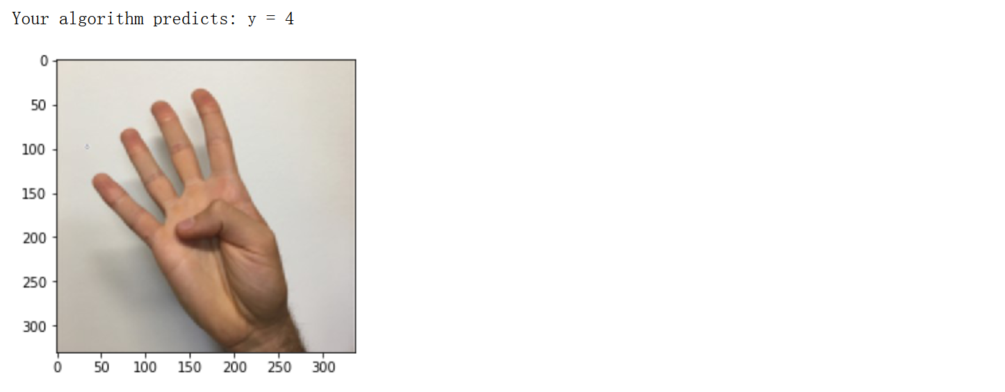
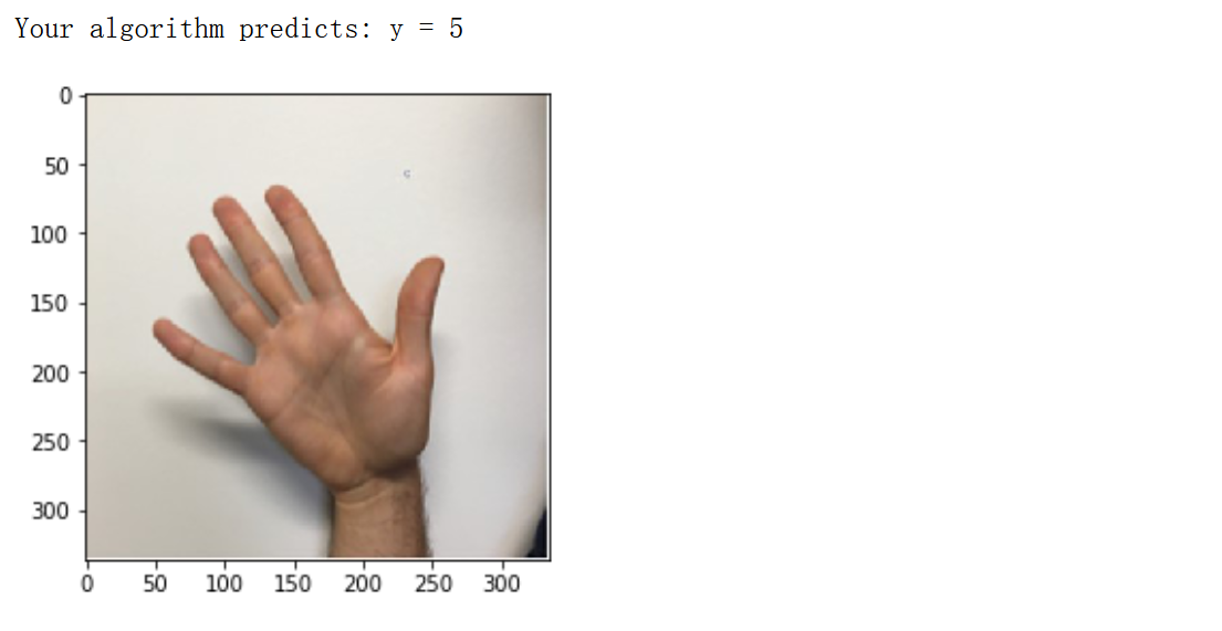
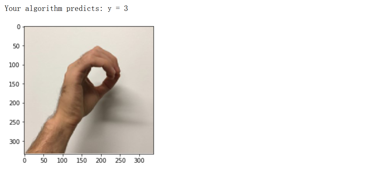
我是否使用了一张看起来像训练集的图片来进行图像测试?也就是说,可以识别截断的图1-5,但仍然无法识别0。
[En]
Did I use a picture that looks like a training set for image testing? That is, the truncated figure 1-5 can be identified, but 0 is still not recognized.

Original: https://blog.csdn.net/weixin_45985148/article/details/123673635
Author: Cary.
Title: 吴恩达深度学习课后作业course2第三周 超参数调试、Batch正则化和程序框架
原创文章受到原创版权保护。转载请注明出处:https://www.johngo689.com/509147/
转载文章受原作者版权保护。转载请注明原作者出处!