

深度学习笔记:从YOLOv5源码loss.py详细介绍Yolov5的损失函数
前言
前一篇博客已经从源码yolo.py介绍了Yolov5的网络结构,这篇文章将从loss.py介绍yolov5的损失函数。
源码的版本是tagV5.0。
class ComputeLoss主要代码分析
1 __init__函数
代码和注释如下:
  def __init__(self, model, autobalance=False):
        super(ComputeLoss, self).__init__()
        device = next(model.parameters()).device
        h = model.hyp

        '''
        定义分类损失和置信度损失为带sigmoid的二值交叉熵损失,
        即会先将输入进行sigmoid再计算BinaryCrossEntropyLoss(BCELoss)。
        pos_weight参数是正样本损失的权重参数。
        '''

        BCEcls = nn.BCEWithLogitsLoss(pos_weight=torch.tensor([h['cls_pw']], device=device))
        BCEobj = nn.BCEWithLogitsLoss(pos_weight=torch.tensor([h['obj_pw']], device=device))

        '''
        对标签做平滑,eps=0就代表不做标签平滑,那么默认cp=1,cn=0
        后续对正类别赋值cp,负类别赋值cn
        '''

        self.cp, self.cn = smooth_BCE(eps=h.get('label_smoothing', 0.0))

        '''
        超参设置g>0则计算FocalLoss
        '''

        g = h['fl_gamma']
        if g > 0:
            BCEcls, BCEobj = FocalLoss(BCEcls, g), FocalLoss(BCEobj, g)

        '''
        获取detect层
        '''
        det = model.module.model[-1] if is_parallel(model) else model.model[-1]
        '''
        每一层预测值所占的权重比,分别代表浅层到深层,小特征到大特征,4.0对应着P3,1.0对应P4,0.4对应P5。
        如果是自己设置的输出不是3层,则返回[4.0, 1.0, 0.25, 0.06, .02],可对应1-5个输出层P3-P7的情况。
        '''
        self.balance = {3: [4.0, 1.0, 0.4]}.get(det.nl, [4.0, 1.0, 0.25, 0.06, .02])
        '''
        autobalance 默认为 False,yolov5中目前也没有使用 ssi = 0即可
        '''
        self.ssi = list(det.stride).index(16) if autobalance else 0
        '''
        赋值各种参数,gr是用来设置IoU的值在objectness loss中做标签的系数,
        使用代码如下:
        tobj[b, a, gj, gi] = (1.0 - self.gr) + self.gr * iou.detach().clamp(0).type(tobj.dtype)  # iou ratio
        train.py源码中model.gr=1,也就是说完全使用标签框与预测框的CIoU值来作为该预测框的objectness标签。
        '''
        self.BCEcls, self.BCEobj, self.gr, self.hyp, self.autobalance = BCEcls, BCEobj, model.gr, h, autobalance
        for k in 'na', 'nc', 'nl', 'anchors':
            setattr(self, k, getattr(det, k))
2 build_targets函数
代码和注释如下:
def build_targets(self, p, targets):

        '''
        na = 3,表示每个预测层anchors的个数
        targets 为一个batch中所有的标签,包括标签所属的image,以及class,x,y,w,h
        targets = [[image1,class1,x1,y1,w1,h1],
                   [image2,class2,x2,y2,w2,h2],
                   ...

                   [imageN,classN,xN,yN,wN,hN]]
        nt为一个batch中所有标签的数量
        '''
        na, nt = self.na, targets.shape[0]
        tcls, tbox, indices, anch = [], [], [], []
        '''
        gain是为了最终将坐标所属grid坐标限制在坐标系内,不要超出范围,
        其中7是为了对应: image class x y w h ai,
        但后续代码只对x y w h赋值,x,y,w,h = nx,ny,nx,ny,
        nx和ny为当前输出层的grid大小。
        '''
        gain = torch.ones(7, device=targets.device)
        '''
        ai.shape = [na,nt]
        ai = [[0,0,0,.....],
              [1,1,1,...],
              [2,2,2,...]]
        这么做的目的是为了给targets增加一个属性,即当前标签所属的anchor索引
        '''
        ai = torch.arange(na, device=targets.device).float().view(na, 1).repeat(1, nt)
        '''
        targets.repeat(na, 1, 1).shape = [na,nt,6]
        ai[:, :, None].shape = [na,nt,1](None在list中的作用就是在插入维度1)
        ai[:, :, None] = [[[0],[0],[0],.....],
                          [[1],[1],[1],...],
                          [[2],[2],[2],...]]
        cat之后:
        targets.shape = [na,nt,7]
        targets = [[[image1,class1,x1,y1,w1,h1,0],
                    [image2,class2,x2,y2,w2,h2,0],
                    ...

                    [imageN,classN,xN,yN,wN,hN,0]],
                    [[image1,class1,x1,y1,w1,h1,1],
                     [image2,class2,x2,y2,w2,h2,1],
                    ...],
                    [[image1,class1,x1,y1,w1,h1,2],
                     [image2,class2,x2,y2,w2,h2,2],
                    ...]]
        这么做是为了纪录每个label对应的anchor。
        '''
        targets = torch.cat((targets.repeat(na, 1, 1), ai[:, :, None]), 2)

        '''
        定义每个grid偏移量,会根据标签在grid中的相对位置来进行偏移
        '''
        g = 0.5
        '''
        [0, 0]代表中间,
        [1, 0] * g = [0.5, 0]代表往左偏移半个grid, [0, 1]*0.5 = [0, 0.5]代表往上偏移半个grid,与后面代码的j,k对应
        [-1, 0] * g = [-0.5, 0]代代表往右偏移半个grid, [0, -1]*0.5 = [0, -0.5]代表往下偏移半个grid,与后面代码的l,m对应
        具体原理在代码后讲述
        '''
        off = torch.tensor([[0, 0],
                            [1, 0], [0, 1], [-1, 0], [0, -1],

                            ], device=targets.device).float() * g

        for i in range(self.nl):
            '''
            原本yaml中加载的anchors.shape = [3,6],但在yolo.py的Detect中已经通过代码
            a = torch.tensor(anchors).float().view(self.nl, -1, 2)
            self.register_buffer('anchors', a)
            将anchors进行了reshape。
            self.anchors.shape = [3,3,2]
            anchors.shape = [3,2]
            '''
            anchors = self.anchors[i]
            '''
            p.shape = [nl,bs,na,nx,ny,no]
            p[i].shape = [bs,na,nx,ny,no]
            gain = [1,1,nx,ny,nx,ny,1]
            '''
            gain[2:6] = torch.tensor(p[i].shape)[[3, 2, 3, 2]]

            '''
            因为targets进行了归一化,默认在w = 1, h =1 的坐标系中,
            需要将其映射到当前输出层w = nx, h = ny的坐标系中。
            '''
            t = targets * gain
            if nt:

                '''
                t[:, :, 4:6].shape = [na,nt,2] = [3,nt,2],存放的是标签的w和h
                anchor[:,None] = [3,1,2]
                r.shape = [3,nt,2],存放的是标签和当前层anchor的长宽比
                '''
                r = t[:, :, 4:6] / anchors[:, None]
                '''
                torch.max(r, 1. / r)求出最大的宽比和最大的长比,shape = [3,nt,2]
                再max(2)求出同一标签中宽比和长比较大的一个,shape = [2,3,nt],之所以第一个维度变成2,
                因为torch.max如果不是比较两个tensor的大小,而是比较1个tensor某一维度的大小,则会返回values和indices:
                    torch.return_types.max(
                        values=tensor([...]),
                        indices=tensor([...]))
                所以还需要加上索引0获取values,
                torch.max(r, 1. / r).max(2)[0].shape = [3,nt],
                将其和hyp.yaml中的anchor_t超参比较,小于该值则认为标签属于当前输出层的anchor
                j = [[bool,bool,....],[bool,bool,...],[bool,bool,...]]
                j.shape = [3,nt]
                '''
                j = torch.max(r, 1. / r).max(2)[0] < self.hyp['anchor_t']

                '''
                t.shape = [na,nt,7]
                j.shape = [3,nt]
                假设j中有NTrue个True值,则
                t[j].shape = [NTrue,7]
                返回的是na*nt的标签中,所有属于当前层anchor的标签。
                '''
                t = t[j]

                '''
                下面这段代码和注释可以配合代码后的图片进行理解。
                t.shape = [NTrue,7]
                7:image,class,x,y,h,w,ai
                gxy.shape = [NTrue,2] 存放的是x,y,相当于坐标到坐标系左边框和上边框的记录
                gxi.shape = [NTrue,2] 存放的是w-x,h-y,相当于测量坐标到坐标系右边框和下边框的距离
                '''
                gxy = t[:, 2:4]
                gxi = gain[[2, 3]] - gxy
                '''
                因为grid单位为1,共nx*ny个gird
                gxy % 1相当于求得标签在第gxy.long()个grid中以grid左上角为原点的相对坐标,
                gxi % 1相当于求得标签在第gxy.long()个grid中以grid右下角为原点的相对坐标,
                下面这两行代码作用在于
                筛选中心坐标 左、上方偏移量小于0.5,并且中心点大于1的标签
                筛选中心坐标 右、下方偏移量小于0.5,并且中心点大于1的标签
                j.shape = [NTrue], j = [bool,bool,...]
                k.shape = [NTrue], k = [bool,bool,...]
                l.shape = [NTrue], l = [bool,bool,...]
                m.shape = [NTrue], m = [bool,bool,...]
                '''
                j, k = ((gxy % 1. < g) & (gxy > 1.)).T
                l, m = ((gxi % 1. < g) & (gxi > 1.)).T
                '''
                j.shape = [5,NTrue]
                t.repeat之后shape为[5,NTrue,7],
                通过索引j后t.shape = [NOff,7],NOff表示NTrue + (j,k,l,m中True的总数量)
                torch.zeros_like(gxy)[None].shape = [1,NTrue,2]
                off[:, None].shape = [5,1,2]
                相加之和shape = [5,NTrue,2]
                通过索引j后offsets.shape = [NOff,2]
                这段代码的表示当标签在grid左侧半部分时,会将标签往左偏移0.5个grid,上下右同理。
                '''
                j = torch.stack((torch.ones_like(j), j, k, l, m))
                t = t.repeat((5, 1, 1))[j]
                offsets = (torch.zeros_like(gxy)[None] + off[:, None])[j]
            else:
                t = targets[0]
                offsets = 0

            '''
            t.shape = [NOff,7],(image,class,x,y,w,h,ai)
            '''
            b, c = t[:, :2].long().T
            gxy = t[:, 2:4]
            gwh = t[:, 4:6]
            '''
            offsets.shape = [NOff,2]
            gxy - offsets为gxy偏移后的坐标,
            gxi通过long()得到偏移后坐标所在的grid坐标
            '''
            gij = (gxy - offsets).long()
            gi, gj = gij.T

            '''
            a:所有anchor的索引 shape = [NOff]
            b:标签所属image的索引 shape = [NOff]
            gj.clamp_(0, gain[3] - 1)将标签所在grid的y限定在0到ny-1之间
            gi.clamp_(0, gain[2] - 1)将标签所在grid的x限定在0到nx-1之间
            indices = [image, anchor, gridy, gridx] 最终shape = [nl,4,NOff]
            tbox存放的是标签在所在grid内的相对坐标,∈[0,1] 最终shape = [nl,NOff]
            anch存放的是anchors 最终shape = [nl,NOff,2]
            tcls存放的是标签的分类 最终shape = [nl,NOff]
            '''
            a = t[:, 6].long()
            indices.append((b, a, gj.clamp_(0, gain[3] - 1), gi.clamp_(0, gain[2] - 1)))
            tbox.append(torch.cat((gxy - gij, gwh), 1))
            anch.append(anchors[a])
            tcls.append(c)

        return tcls, tbox, indices, anch
在上述论文中的代码中包含了标签偏移的代码部分:
   g = 0.5
   off = torch.tensor([[0, 0],
                  [1, 0], [0, 1], [-1, 0], [0, -1],

                  ], device=targets.device).float() * g

  gxy = t[:, 2:4]
  gxi = gain[[2, 3]] - gxy
  j, k = ((gxy % 1. < g) & (gxy > 1.)).T
  l, m = ((gxi % 1. < g) & (gxi > 1.)).T
  j = torch.stack((torch.ones_like(j), j, k, l, m))
  t = t.repeat((5, 1, 1))[j]
  offsets = (torch.zeros_like(gxy)[None] + off[:, None])[j]
  gxy = t[:, 2:4]
  gij = (gxy - offsets).long()
在讲述yolo.py的时候也已经介绍过,这里再介绍一遍。
这段代码的大致意思是,当标签在grid左侧半部分时,会将标签往左偏移0.5个grid,在上、下、右侧同理。具体如图所示:
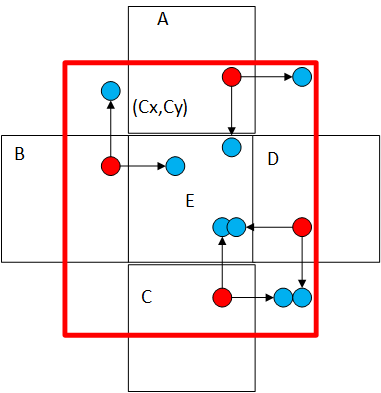

grid B中的标签在右上半部分,所以标签偏移0.5个gird到E中,A,B,C,D同理,即每个网格除了回归中心点在该网格的目标,还会回归中心点在该网格附近周围网格的目标。以E左上角为坐标(Cx,Cy),所以bx∈[Cx-0.5,Cx+1.5],by∈[Cy-0.5,Cy+1.5],而bw∈[0,4pw],bh∈[0,4ph]应该是为了限制anchor的大小。
3 _call__函数
代码和注释如下:
def __call__(self, p, targets):
        device = targets.device
        lcls, lbox, lobj = torch.zeros(1, device=device), torch.zeros(1, device=device), torch.zeros(1, device=device)
        '''
        从build_targets函数中构建目标标签,获取标签中的tcls, tbox, indices, anchors
        tcls = [[cls1,cls2,...],[cls1,cls2,...],[cls1,cls2,...]]
        tcls.shape = [nl,N]
        tbox = [[[gx1,gy1,gw1,gh1],[gx2,gy2,gw2,gh2],...],

        indices = [[image indices1,anchor indices1,gridj1,gridi1],
                   [image indices2,anchor indices2,gridj2,gridi2],
                   ...]]
        anchors = [[aw1,ah1],[aw2,ah2],...]
        '''
        tcls, tbox, indices, anchors = self.build_targets(p, targets)

        '''
        p.shape = [nl,bs,na,nx,ny,no]
        nl 为 预测层数,一般为3
        na 为 每层预测层的anchor数,一般为3
        nx,ny 为 grid的w和h
        no 为 输出数,为5 + nc (5:x,y,w,h,obj,nc:分类数)
        '''
        for i, pi in enumerate(p):
            '''
            a:所有anchor的索引
            b:标签所属image的索引
            gridy:标签所在grid的y,在0到ny-1之间
            gridy:标签所在grid的x,在0到nx-1之间
            '''
            b, a, gj, gi = indices[i]
            '''
            pi.shape = [bs,na,nx,ny,no]
            tobj.shape = [bs,na,nx,ny]
            '''
            tobj = torch.zeros_like(pi[..., 0], device=device)

            n = b.shape[0]
            if n:
                '''
                ps为batch中第b个图像第a个anchor的第gj行第gi列的output
                ps.shape = [N,5+nc],N = a[0].shape,即符合anchor大小的所有标签数
                '''
                ps = pi[b, a, gj, gi]

                '''
                xy的预测范围为-0.5~1.5
                wh的预测范围是0~4倍anchor的w和h,
                原理在代码后讲述。
                '''

                pxy = ps[:, :2].sigmoid() * 2. - 0.5
                pwh = (ps[:, 2:4].sigmoid() * 2) ** 2 * anchors[i]
                pbox = torch.cat((pxy, pwh), 1)
                '''
                只有当CIOU=True时,才计算CIOU,否则默认为GIOU
                '''
                iou = bbox_iou(pbox.T, tbox[i], x1y1x2y2=False, CIoU=True)
                lbox += (1.0 - iou).mean()

                '''
                通过gr用来设置IoU的值在objectness loss中做标签的比重,
                '''
                tobj[b, a, gj, gi] = (1.0 - self.gr) + self.gr * iou.detach().clamp(0).type(tobj.dtype)

                if self.nc > 1:
                    '''
                    ps[:, 5:].shape = [N,nc],用 self.cn 来填充型为[N,nc]得Tensor。
                    self.cn通过smooth_BCE平滑标签得到的,使得负样本不再是0,而是0.5 * eps
                    '''
                    t = torch.full_like(ps[:, 5:], self.cn, device=device)
                    '''
                    self.cp 是通过smooth_BCE平滑标签得到的,使得正样本不再是1,而是1.0 - 0.5 * eps
                    '''
                    t[range(n), tcls[i]] = self.cp
                    '''
                    计算用sigmoid+BCE分类损失
                    '''
                    lcls += self.BCEcls(ps[:, 5:], t)

            '''
            pi[..., 4]所存储的是预测的obj
            '''
            obji = self.BCEobj(c, tobj)
            '''
            self.balance[i]为第i层输出层所占的权重,在init函数中已介绍
            将每层的损失乘上权重计算得到obj损失
            '''
            lobj += obji * self.balance[i]
            if self.autobalance:
                self.balance[i] = self.balance[i] * 0.9999 + 0.0001 / obji.detach().item()

        if self.autobalance:
            self.balance = [x / self.balance[self.ssi] for x in self.balance]
        '''
        hyp.yaml中设置了每种损失所占比重,分别对应相乘
        '''
        lbox *= self.hyp['box']
        lobj *= self.hyp['obj']
        lcls *= self.hyp['cls']
        bs = tobj.shape[0]

        loss = lbox + lobj + lcls
        return loss * bs, torch.cat((lbox, lobj, lcls, loss)).detach()
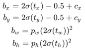
在anchor回归时,对xywh进行了以下处理:
 pxy = ps[:, :2].sigmoid() * 2. - 0.5
 pwh = (ps[:, 2:4].sigmoid() * 2) ** 2 * anchors[i]
这和yolo.py Detect中的代码一致:
y = x[i].sigmoid()
y[..., 0:2] = (y[..., 0:2] * 2. - 0.5 + self.grid[i]) * self.stride[i]
y[..., 2:4] = (y[..., 2:4] * 2) ** 2 * self.anchor_grid[i]
可以先翻看yolov3论文中对于anchor box回归的介绍:
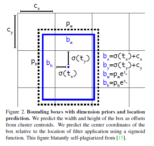
这里的bx∈[Cx,Cx+1],by∈[Cy,Cy+1],bw∈(0,+∞),bh∈(0,+∞)
而yolov5里这段公式变成了:
使得bx∈[Cx-0.5,Cx+1.5],by∈[Cy-0.5,Cy+1.5],bw∈[0,4pw],bh∈[0,4ph]。
这么做是为了消除网格敏感,因为sigmoid函数想取到0或1需要趋于正负无穷,这对网络训练来说是比较难取到的,所以通过往外扩大半个格子范围,是的格点边缘上的点也能取到。
这一策略可以提高召回率(因为每个grid的预测范围变大了),但会略微降低精确度,总体提升mAP。
Original: https://blog.csdn.net/Z960515/article/details/122357364
Author: HollowKnightZ
Title: 从YOLOv5源码loss.py详细介绍Yolov5的损失函数
原创文章受到原创版权保护。转载请注明出处:https://www.johngo689.com/708739/
转载文章受原作者版权保护。转载请注明原作者出处!