

Pytorch 学习笔记-自定义激活函数
*
– 0.激活函数的反向传播
–
+ 1.Relu
+ 2.LeakyRelu
+ 3.Softplus
– 1.Variable与Function(自动梯度计算)
–
+ 0.本章内容
+ 1. pytorch如何构建计算图(Variable与Function)
+ 2. Variable与Tensor差别
+ 3. 动态图机制是如何进行的(Variable和Function的关系)
+ 4.PyTorch中Variable的使用方法
+ 5. Variable的require_grad与volatile参数
+ 6. 对计算图进行可视化
+ 7. 例子
– 2.自定义torch.autograd.Function
–
+ 0.本章内容
+ 1.对Function的直观理解
+ 2. Function与Module的差异与应用场景
+ 3. 一个ReLU Function
+
* 3.1 定义一个ReLU类
*
– 3.1.1 定义一个ReLU类
– 3.1.2 pytorch中关于ctx.save_for_backward()函数的困惑?
* 3.2 验证Variable
* 3.3 Wrap一个ReLU函数
引用:
https://zhuanlan.zhihu.com/p/27147968
浅谈Pytorch中的Variable的使用方法 https://blog.csdn.net/weixin_42782150/article/details/106854349
前向传播(forward)和反向传播(backward)
https://zhuanlan.zhihu.com/p/447113449
激活函数的反向传播
https://blog.csdn.net/csuyzt/article/details/82320589
Pytorch笔记04-自定义torch.autograd.Function
https://zhuanlan.zhihu.com/p/27783097
megengine.org.cn源代码
https://megengine.org.cn/doc/stable/zh/reference/api/megengine.functional.nn.softplus.html
0.激活函数的反向传播
1.Relu


代码实现:
新版本的Function格式
class MyReLU(torch.autograd.Function):
    @staticmethod
    def forward(ctx, input_):

        ctx.save_for_backward(input_)
        output = input_.clamp(min=0)
        return output
    @staticmethod
    def backward(ctx, grad_output):

        input_,  = ctx.saved_tensors
        grad_input = grad_output.clone()
        grad_input[input_ < 0] = 0
        return grad_input
def relu(input_):

    return MyReLU().apply(input_)

老版本的Function格式
import torch
from torch.autograd import Variable

class MyReLU(torch.autograd.Function):

    def forward(self, input_):

        self.save_for_backward(input_)
        output = input_.clamp(min=0)
        return output

    def backward(self, grad_output):

        input_, = self.saved_tensors
        grad_input = grad_output.clone()
        grad_input[input < 0] = 0
        return grad_input
2.LeakyRelu

; 3.Softplus
Softplus 函数
softplus是sigmoid和tanh出现之后提出的一个替代方案,它的函数形式是:

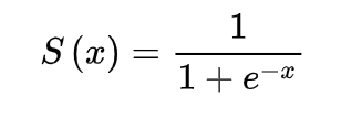
这个函数它完成了对低于阈值部分的抑制(小于0)和大于0部分的激活。在两部分内都是可导的且梯度恒等,这就解决了梯度消失的问题(需要注意这里值域是零到正无穷,因此通常无法用于输出层)。当时softplus函数在反向传播时计算耗费较大,所以应用不是特别广。

def softplus(inp: Tensor) -> Tensor:
    r"""Applies the element-wise function:

    .. math::
        \text{softplus}(x) = \log(1 + \exp(x))

    softplus is a smooth approximation to the ReLU function and can be used
    to constrain the output to be always positive.

    For numerical stability the implementation follows this transformation:

    .. math::
        \text{softplus}(x) = \log(1 + \exp(x))
                           = \log(1 + \exp(-\text{abs}(x))) + \max(x, 0)
                           = \log1p(\exp(-\text{abs}(x))) + \text{relu}(x)

   Examples:

        .. testcode::

            import numpy as np
            from megengine import tensor
            import megengine.functional as F

            x = tensor(np.arange(-3, 3, dtype=np.float32))
            y = F.softplus(x)
            print(y.numpy().round(decimals=4))

        Outputs:

        .. testoutput::

            [0.0486 0.1269 0.3133 0.6931 1.3133 2.1269]
"""
    return log1p(exp(-abs(inp))) + relu(inp)
代码实现:
记住,torch.log 和 torch.exp不能换成math,torch可以对所有的元素单独的运算!nice!

class MySoftplus(torch.autograd.Function):

    @staticmethod
    def forward(ctx, input_):

        ctx.save_for_backward(input_)

        output = torch.log(0.0000000005 + torch.exp(input_))

        return output
    @staticmethod
    def backward(ctx, grad_output):

        input_,  = ctx.saved_tensors
        grad_input1 = grad_output.clone()

        grad_input = grad_input1 * 1/(1+0.0000000005/torch.exp(input_))
        return grad_input

import torch
import math
from torch.autograd import Variable

class MySoftPlus(torch.autograd.Function):

    def forward(self, input_):

        self.save_for_backward(input_)

        self.a=0.0000000005
        output =  math.log(self.a+math.exp(x))
        return output

    def backward(self, grad_output):

        input_, = self.saved_tensors
        grad_input_1 = grad_output.clone()
        grad_input = grad_input_1 * 1/(1+self.a/math.exp(input_))
        return grad_input
    def forward_fuse(self, x):
         print(11111111,MySoftplus.apply((self.conv1(x)) + MySoftplus.apply(self.conv2(x))) )

         print(MySoftplus.apply((self.conv1(x)) + MySoftplus.apply(self.conv2(x)))-MySoftplus.apply((self.conv1(x)) + self.conv2(x)))
         return MySoftplus.apply((self.conv1(x)) + MySoftplus.apply(self.conv2(x)))

         return MySoftplus.apply((self.conv1(x)) + self.conv2(x))
1.Variable与Function(自动梯度计算)
0.本章内容
pytorch的自动梯度计算是基于其中的Variable类和Function类构建计算图,在本章中将介绍如何生成计算图,以及pytorch是如何进行反向传播求梯度的,主要内容如下:
pytorch如何构建计算图( Variable与 Function类)
Variable与 Tensor的差别
动态图机制是如何进行的( Variable与 Function如何建立计算图)
Variable的基本操作
Variable的require_grad与volatile参数
对计算图进行可视化
所有源码都能在XavierLinNow/pytorch_note_CN这里获取
1. pytorch如何构建计算图( Variable 与 Function )
一般一个神经网络都可以用一个有向无环图图来表示计算过程,在pytorch中也是构建计算图来实现forward计算以及backward梯度计算。
计算图由节点和边组成。
计算图中边相当于一种函数变换或者说运算,节点表示参与运算的数据。边上两端的两个节点中,一个为函数的输入数据,一个为函数的输出数据。
而 Variable就相当于计算图中的节点。
Function就相当于是计算图中的边,它实现了对一个输入 Variable变换为另一个输出的 Variable
因此, Variable需要保存forward时计算的激活值。这个值是一个 Tensor,可以通过 .data来得到这个Variable所保存的forward时的计算值。
同时反向传导时,一个 Variable还需要保存其梯度。该梯度也是一个 Variable,可以通过 .grad来得到。== (目前我认为是对下一个神经元的梯度贡献,比如output = torch.sum(3 x),就相当于output=3(x11+x12+…+x21+x22+…),求导之后就是对于xij,梯度是3*1,所以x.grad=[[3,3],[3,3]]这种形式,Variable才有grad操作,tensor没有!) ==
2. Variable与Tensor差别

Tensor只是一个类似 Numpy array的数据格式,它可以进行多种运行,但无法构建计算图
Variable不仅封装了 Tensor作为对应的激活值,还保存了产生这个 Variable的 Function(即计算图中的边),可以通过 .creator(见图)来看是哪个Function输出了这个Variable
在forward时, Variable和 Function构建一个计算图。只有得到了计算图,构建了 Variable与 Function与Variable的输入输出关系,才能在backward时,计算各个节点的梯度。
Variable可以进行 Tensor的大部分计算
对 Variable使用 .backward()方法,可以得到该Variable之前计算图所有Variable的梯度
Variable.data是该Variable前向传播的激活值,为一个Tensor
Variable.grad是该Variable后向传播的值,为一个Variable
; 3. 动态图机制是如何进行的(Variable和Function的关系)
Variable与Function组成了计算图
Function是在每次对Variable进行运算生成的,表示的是该次运算
动态图是在每次forward时动态生成的。具体说,假如有Variable x,Function 。他们需要进行运算y = x * x,则在运算过程时生成得到一个动态图,该动态图输入是x,输出是y,y的 .creator 是
一次forward过程将有多个Function连接各个Variable,Function输出的Variable将保存该Function的引用(即.creator),从而组成计算图
在backward时,将利用生成的计算图,根据求导的链式法则得到每个Variable的梯度值
4.PyTorch中Variable的使用方法
Variable一般的初始化方法,默认是不求梯度的。
import torch
from torch.autograd import Variable

x_tensor = torch.randn(2,3)

x = Variable(x_tensor)
print(x.requires_grad)
>>>
False

x = Variable(x_tensor,requires_grad=True)
print(x)
>>>
tensor([[0.1163, 0.7213, 0.5636],
        [1.1431, 0.8590, 0.7056]], requires_grad=True)
典型范例:
import torch
from torch.autograd import Variable
tensor = torch.FloatTensor([[1,2], [3,4]])
print(tensor)
>>>
tensor([[1., 2.],
        [3., 4.]])
variable = Variable(tensor, requires_grad=True)
print(variable)
>>>
tensor([[1., 2.],
        [3., 4.]], requires_grad=True)

t_out = torch.mean(tensor*tensor)
print(t_out)
>>>
tensor(7.5000)

v_out = torch.mean(variable*variable)
print(v_out)
>>>
tensor(7.5000, grad_fn=<MeanBackward0>)

v_out.backward()
print(variable.grad)
>>>
tensor([[0.5000, 1.0000],
        [1.5000, 2.0000]])

=========================================

x = Variable(torch.ones([1]), requires_grad=True)
y = 0.5 * (x + 1).pow(2)
z = torch.log(y)

z.backward()
print(x.grad)

print(y.grad)
5. Variable的require_grad与volatile参数
在创建一个Variable是,有两个bool型参数可供选择,一个是requires_grad,一个是Volatile
requires_grad不是十分对该Var进行计算梯度,一般在finetune是可以用来固定某些层的参数,减少计算。只要有一个叶节点是True,其后续的节点都是True
volatile=True,一般用在训练好网络,只进行inference操作时使用,其不建立Variable与Function的关系。只要有一个叶子节点是True,其后节点都是True
6. 对计算图进行可视化
7. 例子
我们同样用一个简单的例子来说明如何使用Variable,在引入Variable后,我们已经不需要自己手动计算梯度了
from sklearn.datasets import load_boston
from sklearn import preprocessing
from torch.autograd import Variable

dtype = torch.cuda.FloatTensor
X, y = load_boston(return_X_y=True)
X = preprocessing.scale(X[:100,:])
y = preprocessing.scale(y[:100].reshape(-1, 1))

data_size, D_input, D_output, D_hidden = X.shape[0], X.shape[1], 1, 50
X = Variable(torch.Tensor(X).type(dtype), requires_grad=False)
y = Variable(torch.Tensor(y).type(dtype), requires_grad=False)
w1 = Variable(torch.randn(D_input, D_hidden).type(dtype), requires_grad=True)
w2 = Variable(torch.randn(D_hidden, D_output).type(dtype), requires_grad=True)

lr = 1e-5
epoch = 200000
for i in range(epoch):

    h = torch.mm(X, w1)
    h_relu = h.clamp(min=0)
    y_pred = torch.mm(h_relu, w2)
    loss = (y_pred - y).pow(2).sum()
    if i % 10000 == 0:
        print('epoch: {} loss: {}'.format(i, loss.data[0]))

    loss.backward()

    w1.data -= lr * w1.grad.data
    w2.data -= lr * w2.grad.data

    w1.grad.data.zero_()
    w2.grad.data.zero_()
import torch
from torch.autograd import Variable

x = Variable(torch.ones(2,2), requires_grad=True)
print(x)
>>>
tensor([[1., 1.],
        [1., 1.]], requires_grad=True)

y = x+2
print(y)
>>>
tensor([[3., 3.],
        [3., 3.]], grad_fn=<AddBackward0>)
print(y.grad_fn)
>>>
<AddBackward0 object at 0x12b804510>

z = y * y * 4
out = z.mean()
print("z:{}\nout:{}\n".format(z, out))
>>>
z:tensor([[36., 36.],
        [36., 36.]], grad_fn=<MulBackward0>)
out:36.0

out.backward()
print(x.grad)
>>>
tensor([[6., 6.],
        [6., 6.]])
2.自定义torch.autograd.Function
0.本章内容
在本次,我们将学习如何自定义一个torch.autograd.Function,下面是本次的主要内容
- 对Function的直观理解
- Function与Module的差异与应用场景
- 写一个简单的ReLU Function
1.对Function的直观理解
- 在之前的介绍中,我们知道,Pytorch是利用Variable与Function来构建计算图的。回顾下Variable,Variable就像是计算图中的节点,保存计算结果(包括前向传播的激活值,反向传播的梯度),而Function就像计算图中的边,实现Variable的计算,并输出新的Variable
- Function简单说就是对Variable的运算,如加减乘除,relu,pool等
- 但它不仅仅是简单的运算。与普通Python或者numpy的运算不同,Function是针对计算图,需要计算反向传播的梯度。因此他不仅需要进行该运算(forward过程),还需要保留前向传播的输入(为计算梯度),并支持反向传播计算梯度。如果有做过公开课cs231的作业,记得里面的每个运算都定义了forward,backward,并通过保存cache来进行反向传播。这两者是类似的。
- 在之前Variable的学习中,我们知道进行一次运算后,输出的Variable对应的creator就是其运行的计算,如y = relu(x), y.creator,就是relu这个Function
- 我们可以对Function进行拓展,使其满足我们自己的需要,而拓展就需要自定义Function的forward运算,已经对应的backward运算,同时在forward中需要通过保存输入值用于backward
- 总结,Function与Variable构成了pytorch的自动求导机制,它定义的是各个Variable之间的计算关系
2. Function与Module的差异与应用场景
Function与Module都可以对pytorch进行自定义拓展,使其满足网络的需求,但这两者还是有十分重要的不同:
- Function一般只定义一个操作,因为其无法保存参数,因此适用于激活函数、pooling等操作;Module是保存了参数,因此适合于定义一层,如线性层,卷积层,也适用于定义一个网络
- Function需要定义三个方法: init, forward, backward(需要自己写求导公式);Module:只需定义__init__和forward,而backward的计算由自动求导机制构成
- 可以不严谨的认为,Module是由一系列Function组成,因此其在forward的过程中,Function和Variable组成了计算图,在backward时,只需调用Function的backward就得到结果,因此Module不需要再定义backward。
- Module不仅包括了Function,还包括了对应的参数,以及其他函数与变量,这是Function所不具备的
3. 一个ReLU Function
- 首先我们定义一个继承Function的ReLU类
- 然后我们来看Variable在进行运算时,其creator是否是对应的Function
- 最后我们为方便使用这个ReLU类,将其wrap成一个函数,方便调用,不必每次显式都创建一个新对象
3.1 定义一个ReLU类
3.1.1 定义一个ReLU类
import torch
from torch.autograd import Variable

class MyReLU(torch.autograd.Function):

    def forward(self, input_):

        self.save_for_backward(input_)
        output = input_.clamp(min=0)
        return output

    def backward(self, grad_output):

        input_, = self.saved_tensors
        grad_input = grad_output.clone()
        grad_input[input < 0] = 0
        return grad_input
3.1.2 pytorch中关于ctx.save_for_backward()函数的困惑?
pytorch中在自定义autograd function时,需要编写forward和backward函数,其中经常用到ctx.saved_for_backward()函数。例如:
forward中:ctx.save_for_backward(input)
backward中:input, = ctx.saved_tensors
但是,可以直接写成如下的语句也并没有出现错误:
forward中:ctx.input = input
backward中:input = ctx.input
那么便引出了如下问题:
(1)使用saved_for_backward()是否会copy tensor?使用第二种写法呢(这个没有吧)?
(2)使用saved_for_backward()相比于第二种写法的优势在哪里(尤其在执行效率上)?
(3)使用saved_for_backward()时,保存的是tensor还是Variable(Parameter)?如果是tensor,那么backward()函数中就不需要with torch.nograd()了。
pytorch documentation, pytorch forum以及google上均没有对以上问题给予解答。
saved_for_backward是会保留此input的全部信息(一个完整的外挂Autograd Function的Variable), 并提供避免in-place操作导致的input在backward被修改的情况.而如果在forward中使用 ctx.input = input, 原则上跟官方的例子无甚差别, 差别只在
a check is made to ensure they weren't used in any in-place operation that modified their content.
官方的说明如下:
class _ContextMethodMixin(object):
def save_for_backward(self, *tensors):
r"""Saves given tensors for a future call to :func:~Function.backward.
**This should be called at most once, and only from inside the**
:func:forward **method.**
Later, saved tensors can be accessed through the :attr:saved_tensors
attribute. Before returning them to the user, a check is made to ensure
they weren't used in any in-place operation that modified their content.
Arguments can also be 这里 ctx 相当于 class 中的 self, 这里你可以去 github 看一下 PyTorch 官方源码,有 ctx.save_for_backward 函数的实现。
https://link.zhihu.com/?target=https%3A//github.com/pytorch/pytorch/blob/949d6ae184a15bbed3f30bb0427268c86dc4f5bb/torch/autograd/function.py
可以根据自己使用的 PyTorch 版本,查看对应release的源码。最新版本中,tensor跟Variable合并了,tensor也可以有grad,且ctx.save_for_backward的实现其实就是你所说的 ctx.input = input
3.2 验证Variable
与Function的关系
from torch.autograd import Variable
input_ = Variable(torch.randn(1))
relu = MyReLU()
output_ = relu(input_)

print relu
print output_.creator
输出:
<__main__.myrelu object at 0x7fd0b2d08b30>
<__main__.myrelu object at 0x7fd0b2d08b30>
</__main__.myrelu></__main__.myrelu>
可见,Function连接了Variable与Variable并实现不同计算
3.3 Wrap一个ReLU函数
可以直接把刚才自定义的ReLU类封装成一个函数,方便直接调用
def relu(input_):

    return MyReLU()(input_)
input_ = Variable(torch.linspace(-3, 3, steps=5))
print input_
print relu(input_)
输出:
Variable containing:
-3.0000
-1.5000
 0.0000
 1.5000
 3.0000
[torch.FloatTensor of size 5]

Variable containing:
 0.0000
 0.0000
 0.0000
 1.5000
 3.0000
[torch.FloatTensor of size 5]
Original: https://blog.csdn.net/weixin_49117441/article/details/123056849
Author: @bnu_smile
Title: Pytorch 学习笔记-自定义激活函数
原创文章受到原创版权保护。转载请注明出处:https://www.johngo689.com/707305/
转载文章受原作者版权保护。转载请注明原作者出处!