

(一)银行卡号识别 —— sort_contours()、resize()
【信用卡检测流程详解】
11、提取模板的每个数字
1111、读取模板图像、转换成灰度图、转换成二值图
1122、轮廓检测、绘制轮廓、对得到的所有轮廓进行排序(编号)
1133、提取模板的所有轮廓 – 每一个数字
22、提取信用卡的所有轮廓
2211、读取待检测图像、转换为灰度图、顶帽操作、sobel算子操作、闭操作、二值化、二次膨胀+腐蚀
2222、轮廓检测、绘制轮廓
33、提取银行卡《四个数字一组》轮廓,然后每个轮廓与模板的每一个数字进行匹配,得到最大匹配结果
3311、在所有轮廓中,识别出《四个数字一组》的轮廓(共有四个),并进行阈值化、轮廓检测和轮廓排序
3322、在《四个数字一组》中,提取每个数字的轮廓以及坐标,并进行模板匹配得到最大匹配结果
44、在原图像上,用矩形画出《四个数字一组》,并在原图上显示所有的匹配结果


import cv2
import matplotlib.pyplot as plt
import numpy as np

def sort_contours(cnt_s, method="left-to-right"):
    reverse = False
    ii_myutils = 0
    if method == "right-to-left" or method == "bottom-to-top":
        reverse = True
    if method == "top-to-bottom" or method == "bottom-to-top":
        ii_myutils = 1
    bounding_boxes = [cv2.boundingRect(cc_myutils) for cc_myutils in cnt_s]
    (cnt_s, bounding_boxes) = zip(*sorted(zip(cnt_s, bounding_boxes), key=lambda b: b[1][ii_myutils], reverse=reverse))
    return cnt_s, bounding_boxes

def resize(image, width=None, height=None, inter=cv2.INTER_AREA):
    dim_myutils = None
    (h_myutils, w_myutils) = image.shape[:2]
    if width is None and height is None:
        return image
    if width is None:
        r_myutils = height / float(h_myutils)
        dim_myutils = (int(w_myutils * r_myutils), height)
    else:
        r_myutils = width / float(w_myutils)
        dim_myutils = (width, int(h_myutils * r_myutils))
    resized = cv2.resize(image, dim_myutils, interpolation=inter)
    return resized

img = cv2.imread(r'ocr_a_reference.png')
ref_gray = cv2.cvtColor(img, cv2.COLOR_BGR2GRAY)
ref_BINARY = cv2.threshold(ref_gray, 10, 255, cv2.THRESH_BINARY_INV)[1]
"""#######################################
轮廓检测:contours, hierarchy = cv2.findContours(img, mode, method)
输入参数      mode: 轮廓检索模式
                  (1)RETR_EXTERNAL:  只检索最外面的轮廓;
                  (2)RETR_LIST:      检索所有的轮廓,但检测的轮廓不建立等级关系,将其保存到一条链表当中,
                  (3)RETR_CCOMP:     检索所有的轮廓,并建立两个等级的轮廓。顶层是各部分的外部边界,内层是的边界信息;
                  (4)RETR_TREE:      检索所有的轮廓,并建立一个等级树结构的轮廓;(最常用)
            method: 轮廓逼近方法
                  (1)CHAIN_APPROX_NONE:      存储所有的轮廓点,相邻的两个点的像素位置差不超过1。               例如:矩阵的四条边。(最常用)
                  (2)CHAIN_APPROX_SIMPLE:     压缩水平方向,垂直方向,对角线方向的元素,只保留该方向的终点坐标。   例如:矩形的4个轮廓点。
输出参数     contours:所有的轮廓
            hierarchy:每条轮廓对应的属性
备注0:轮廓就是将连续的点(连着边界)连在一起的曲线,具有相同的颜色或者灰度。轮廓在形状分析和物体的检测和识别中很有用。
备注1:函数输入图像是二值图,即黑白的(不是灰度图)。所以读取的图像要先转成灰度的,再转成二值图。
备注2:函数在opencv2只返回两个值:contours, hierarchy。
备注3:函数在opencv3会返回三个值:img, countours, hierarchy
#######################################"""
refCnts, hierarchy = cv2.findContours(ref_BINARY.copy(), cv2.RETR_EXTERNAL, cv2.CHAIN_APPROX_SIMPLE)

"""#######################################
绘制轮廓:v2.drawContours(image, contours, contourIdx, color, thickness) ———— (在图像上)画出图像的轮廓
输入参数        image:             需要绘制轮廓的目标图像,注意会改变原图
              contours:           轮廓点,上述函数cv2.findContours()的第一个返回值
              contourIdx:         轮廓的索引,表示绘制第几个轮廓。-1表示绘制所有的轮廓
              color:              绘制轮廓的颜色(RGB)
              thickness:          (可选参数)轮廓线的宽度,-1表示填充
备注:图像需要先复制一份copy(), 否则(赋值操作的图像)与原图会随之一起改变。
#######################################"""
img_Contours = img.copy()
cv2.drawContours(img_Contours, refCnts, -1, (0, 0, 255), 3)

plt.subplot(221),   plt.imshow(img, 'gray'),            plt.title('(0)ref')
plt.subplot(222),   plt.imshow(ref_gray, 'gray'),       plt.title('(1)ref_gray')
plt.subplot(223),   plt.imshow(ref_BINARY, 'gray'),     plt.title('(2)ref_BINARY')
plt.subplot(224),   plt.imshow(img_Contours, 'gray'),   plt.title('(3)img_Contours')
plt.show()

refCnts = sort_contours(refCnts, method="left-to-right")[0]

digits = {}
for (i, c) in enumerate(refCnts):
    (x, y, w, h) = cv2.boundingRect(c)
    roi = ref_BINARY[y:y + h, x:x + w]
    roi = cv2.resize(roi, (57, 88))
    digits[i] = roi

"""######################################################################
初始化卷积核:getStructuringElement(shape, ksize)
输入参数:       shape:形状
                        (1) MORPH_RECT          矩形
                        (2) MORPH_CROSS         十字型
                        (3) MORPH_ELLIPSE       椭圆形
                ksize:卷积核大小。例如:(3, 3)表示3*3的卷积核
######################################"""
rect_Kernel = cv2.getStructuringElement(cv2.MORPH_RECT, (9, 3))
square_Kernel = cv2.getStructuringElement(cv2.MORPH_RECT, (5, 5))

image_card = cv2.imread(r'images\credit_card_01.png')
image_resize = resize(image_card, width=300)
image_gray = cv2.cvtColor(image_resize, cv2.COLOR_BGR2GRAY)

"""#######################################
形态学变化函数:cv2.morphologyEx(src, op, kernel)
参数说明:src传入的图片,op进行变化的方式, kernel表示方框的大小
op变化的方式有五种:
        开运算(open):             cv2.MORPH_OPEN              先腐蚀,再膨胀。                  开运算可以用来消除小黑点。
        闭运算(close):            cv2.MORPH_CLOSE             先膨胀,再腐蚀。                  闭运算可以用来突出边缘特征。
        形态学梯度(morph-grad):    cv2.MORPH_GRADIENT          膨胀后图像(减去)腐蚀图像。        可以突出团块(blob)的边缘,保留物体的边缘轮廓。
        顶帽(top-hat):            cv2.MORPH_TOPHAT            原始输入(减去)开运算结果。        将突出比原轮廓亮的部分。
        黑帽(black-hat):          cv2.MORPH_BLACKHAT          闭运算结果(减去)原始输入          将突出比原轮廓暗的部分。
#######################################"""
image_tophat = cv2.morphologyEx(image_gray, cv2.MORPH_TOPHAT, rect_Kernel)

"""#######################################
Sobel算子是一种常用的边缘检测算子。对噪声具有平滑作用,提供较为精确的边缘方向信息,但是边缘定位精度不够高。
        边缘就是像素对应的灰度值快速变化的地方。如:黑到白的边界
        图像是二维的。Sobel算子在x,y两个方向求导,故有不同的两个卷积核(Gx, Gy),且Gx的转置等于Gy。分别反映了每一点像素在水平方向和在垂直方向上的亮度变换情况.

########################################
dst = cv2.Sobel(src, ddepth, dx, dy, ksize)
输入参数    src        输入图像
          ddepth     图像的深度,-1表示采用的是与原图像相同的深度。目标图像的深度必须大于等于原图像的深度;
          dx和dy     表示的是求导的阶数,0表示这个方向上没有求导,一般为0、1、2。
          ksize      卷积核大小,一般为3、5。
同时对x和y进行求导,会导致部分信息丢失。(不建议)- 分别计算x和y,再求和(效果好)
########################################
(1)cv2.CV_16S的说明
      (1)Sobel函数求完导数后会有负值,还有会大于255的值。
      (2)而原图像是uint8,即8位无符号数。所以Sobel建立图像的位数不够,会有截断。
      (3)因此要使用16位有符号的数据类型,即cv2.CV_16S。
(2)cv2.convertScaleAbs(): 给图像的所有像素加一个绝对值
      通过该函数将其转回原来的uint8形式。否则将无法显示图像,而只是一副灰色的窗口。
########################################"""

image_gradx = cv2.Sobel(image_tophat, ddepth=cv2.CV_32F, dx=1, dy=0, ksize=-1)
image_gradx = np.absolute(image_gradx)
(minVal, maxVal) = (np.min(image_gradx), np.max(image_gradx))
image_gradx = (255 * ((image_gradx - minVal) / (maxVal - minVal)))
image_gradx = image_gradx.astype("uint8")
"""
sobel_Gx1 = cv2.Sobel(image_tophat, ddepth=cv2.CV_32F, dx=1, dy=0, ksize=3)     # 3*3卷积核
sobel_Gx_Abs1 = cv2.convertScaleAbs(sobel_Gx1)                                  # (1)左边减右边(2)白到黑是正数,黑到白就是负数,且所有的负数会被截断成0,所以要取绝对值。
sobel_Gy1 = cv2.Sobel(image_tophat, cv2.CV_64F, 0, 1, ksize=3)
sobel_Gy_Abs1 = cv2.convertScaleAbs(sobel_Gy1)
sobel_Gx_Gy_Abs1 = cv2.addWeighted(sobel_Gx_Abs1, 0.5, sobel_Gy_Abs1, 0.5, 0)   # 权重值x + 权重值y +偏置b
"""

image_CLOSE = cv2.morphologyEx(image_gradx, cv2.MORPH_CLOSE, square_Kernel)
"""########################################
图像阈值 ret, dst = cv2.threshold(src, thresh, max_val, type)
输入参数        dst:    输出图
                src:    输入图,只能输入单通道图像,通常来说为灰度图
                thresh:     阈值
                max_val:    当像素值超过了阈值(或者小于阈值,根据type来决定),所赋予的值
                type:       二值化操作的类型,包含以下5种类型:
                    (1) cv2.THRESH_BINARY             超过阈值部分取max_val(最大值),否则取0
                  (2) cv2.THRESH_BINARY_INV         THRESH_BINARY的反转
                    (3) cv2.THRESH_TRUNC              大于阈值部分设为阈值,否则不变
                    (4) cv2.THRESH_TOZERO             大于阈值部分不改变,否则设为0
                    (5) cv2.THRESH_TOZERO_INV         THRESH_TOZERO的反转
########################################"""

image_thresh = cv2.threshold(image_CLOSE, 0, 255, cv2.THRESH_BINARY | cv2.THRESH_OTSU)[1]

image_2_dilate = cv2.dilate(image_thresh, square_Kernel, iterations=2)
image_1_erode = cv2.erode(image_2_dilate, square_Kernel, iterations=1)
image_2_CLOSE = image_1_erode

threshCnts, hierarchy = cv2.findContours(image_2_CLOSE.copy(), cv2.RETR_EXTERNAL, cv2.CHAIN_APPROX_SIMPLE)

image_Contours = image_resize.copy()
cv2.drawContours(image_Contours, threshCnts, -1, (0, 0, 255), 3)

plt.subplot(241),   plt.imshow(image_card, 'gray'),             plt.title('(0)image_card')
plt.subplot(242),   plt.imshow(image_gray, 'gray'),             plt.title('(1)image_gray')
plt.subplot(243),   plt.imshow(image_tophat, 'gray'),           plt.title('(2)image_tophat')
plt.subplot(244),   plt.imshow(image_gradx, 'gray'),            plt.title('(3)image_gradx')
plt.subplot(245),   plt.imshow(image_CLOSE, 'gray'),            plt.title('(4)image_CLOSE')
plt.subplot(246),   plt.imshow(image_thresh, 'gray'),           plt.title('(5)image_thresh')
plt.subplot(247),   plt.imshow(image_2_CLOSE, 'gray'),          plt.title('(6)image_2_CLOSE')
plt.subplot(248),   plt.imshow(image_Contours, 'gray'),         plt.title('(7)image_Contours')
plt.show()

locs = []
for (i, c) in enumerate(threshCnts):
    (x, y, w, h) = cv2.boundingRect(c)
    ar = w / float(h)

    if (2.0 < ar and ar < 4.0):
        if (35 < w < 60) and (10 < h < 20):
            locs.append((x, y, w, h))

locs = sorted(locs, key=lambda x:x[0])

output = []

for (ii, (gX, gY, gW, gH)) in enumerate(locs):
    groupOutput = []

    group_digit = image_gray[gY - 5:gY + gH + 5, gX - 5:gX + gW + 5]
    group_digit_th = cv2.threshold(group_digit, 0, 255, cv2.THRESH_BINARY | cv2.THRESH_OTSU)[1]
    digitCnts, hierarchy = cv2.findContours(group_digit_th.copy(), cv2.RETR_EXTERNAL, cv2.CHAIN_APPROX_SIMPLE)
    digitCnts = sort_contours(digitCnts, method="left-to-right")[0]

    for jj in digitCnts:
        (x, y, w, h) = cv2.boundingRect(jj)
        roi = group_digit[y:y + h, x:x + w]
        roi = cv2.resize(roi, (57, 88))
        cv2.imshow("Image", roi)
        cv2.waitKey(200)
        """########################################
        # 模板匹配:cv2.matchTemplate(image, template, method)
        # 输入参数      image 待检测图像
        #               template 模板图像
        #               method 模板匹配方法:
        #                       (1)cv2.TM_SQDIFF:         计算平方差。          计算出来的值越接近0,越相关
        #                       (2)cv2.TM_CCORR:          计算相关性。          计算出来的值越大,越相关
        #                       (3)cv2.TM_CCOEFF:         计算相关系数。         计算出来的值越大,越相关
        #                       (4)cv2.TM_SQDIFF_NORMED:  计算(归一化)平方差。   计算出来的值越接近0,越相关
        #                       (5)cv2.TM_CCORR_NORMED:   计算(归一化)相关性。   计算出来的值越接近1,越相关
        #                       (6)cv2.TM_CCOEFF_NORMED:  计算(归一化)相关系数。  计算出来的值越接近1,越相关
        # (最好选择有归一化操作,效果好)
        ########################################
        # 获取匹配结果函数:min_val, max_val, min_loc, max_loc = cv2.minMaxLoc(ret)
        # 其中: ret是cv2.matchTemplate函数返回的矩阵;
        #       min_val, max_val, min_loc, max_loc分别表示最小值,最大值,最小值与最大值在图像中的位置
        # 如果模板方法是平方差或者归一化平方差,要用min_loc; 其余用max_loc
        ########################################"""
        scores = []
        for (kk, digitROI) in digits.items():
            result = cv2.matchTemplate(roi, digitROI, cv2.TM_CCOEFF)
            (_, max_score, _, _) = cv2.minMaxLoc(result)
            scores.append(max_score)
        groupOutput.append(str(np.argmax(scores)))
    """########################################
    # 添加文字及修改格式函数:cv2.putText(img, str(i), (123, 456)), font, 2, (0, 255, 0), 3)
    #                    输入参数依次是:图片,添加的文字,左上角坐标,字体,字体大小,颜色,字体粗细
    ########################################"""

    cv2.rectangle(image_resize, (gX - 5, gY - 5), (gX + gW + 5, gY + gH + 5), (0, 0, 255), 1)
    cv2.putText(image_resize, "".join(groupOutput), (gX, gY - 15), cv2.FONT_HERSHEY_SIMPLEX, 0.65, (0, 0, 255), 2)

    output.extend(groupOutput)

cv2.imshow("Image", image_resize)
cv2.waitKey(0)
(二)文档扫描OCR识别 —— cv2.getPerspectiveTransform() + cv2.warpPerspective()、np.argmin()、np.argmax()、np.diff()
计算轮廓的长度:cv2.arcLength(curve, closed)
找出轮廓的多边形拟合曲线:approxPolyDP(contourMat, 10, true)
求最小值对应的索引:np.argmin()
求最大值对应的索引:np.argmax()
求(同一行)列与列之间的差值:np.diff()

import numpy as np
import cv2
import matplotlib.pyplot as plt
"""######################################################################
计算齐次变换矩阵:cv2.getPerspectiveTransform(rect, dst)
输入参数        rect输入图像的四个点(四个角)
                dst输出图像的四个点(方方正正的图像对应的四个角)
######################################################################
仿射变换:cv2.warpPerspective(src, M, dsize, dst=None, flags=None, borderMode=None, borderValue=None)
透视变换:cv2.warpAffine(src, M, dsize, dst=None, flags=None, borderMode=None, borderValue=None)
                src:输入图像     dst:输出图像
                M:2×3的变换矩阵
                dsize:变换后输出图像尺寸
                flag:插值方法
                borderMode:边界像素外扩方式
                borderValue:边界像素插值,默认用0填充
#
(Affine Transformation)可实现旋转,平移,缩放,变换后的平行线依旧平行。
(Perspective Transformation)即以不同视角的同一物体,在像素坐标系中的变换,可保持直线不变形,但是平行线可能不再平行。
#
备注:cv2.warpAffine需要与cv2.getPerspectiveTransform搭配使用。
######################################################################"""

def order_points(pts):
    rect = np.zeros((4, 2), dtype="float32")

    s = pts.sum(axis=1)
    rect[0] = pts[np.argmin(s)]
    rect[2] = pts[np.argmax(s)]

    diff = np.diff(pts, axis=1)
    rect[1] = pts[np.argmin(diff)]
    rect[3] = pts[np.argmax(diff)]
    return rect

def four_point_transform(image, pts):
    rect = order_points(pts)
    (tl, tr, br, bl) = rect

    widthA = np.sqrt(((br[0] - bl[0]) ** 2) + ((br[1] - bl[1]) ** 2))
    widthB = np.sqrt(((tr[0] - tl[0]) ** 2) + ((tr[1] - tl[1]) ** 2))
    maxWidth = max(int(widthA), int(widthB))

    heightA = np.sqrt(((tr[0] - br[0]) ** 2) + ((tr[1] - br[1]) ** 2))
    heightB = np.sqrt(((tl[0] - bl[0]) ** 2) + ((tl[1] - bl[1]) ** 2))
    maxHeight = max(int(heightA), int(heightB))

    dst = np.array([[0, 0], [maxWidth - 1, 0], [maxWidth - 1, maxHeight - 1], [0, maxHeight - 1]], dtype="float32")
    """###############################################################################
    # 计算齐次变换矩阵:cv2.getPerspectiveTransform(rect, dst)
    ###############################################################################"""
    M = cv2.getPerspectiveTransform(rect, dst)

    """###############################################################################
    # 透视变换(将输入矩形乘以(齐次变换矩阵),得到输出矩阵)
    ###############################################################################"""
    warped = cv2.warpPerspective(image, M, (maxWidth, maxHeight))
    return warped

def resize(image, width=None, height=None, inter=cv2.INTER_AREA):
    dim = None
    (h, w) = image.shape[:2]
    if width is None and height is None:
        return image
    if width is None:
        r = height / float(h)
        dim = (int(w * r), height)
    else:
        r = width / float(w)
        dim = (width, int(h * r))
    resized = cv2.resize(image, dim, interpolation=inter)
    return resized

image = cv2.imread(r'images\receipt.jpg')
ratio = image.shape[0] / 500.0
orig = image.copy()
image = resize(orig, height=500)

gray = cv2.cvtColor(image, cv2.COLOR_BGR2GRAY)
gray = cv2.GaussianBlur(gray, (5, 5), 0)
edged = cv2.Canny(gray, 75, 200)

print("STEP 1: 边缘检测")
cv2.imshow("Image", image)
cv2.imshow("Edged", edged)
cv2.waitKey(0)
cv2.destroyAllWindows()

cnts, hierarchy = cv2.findContours(edged.copy(), cv2.RETR_LIST, cv2.CHAIN_APPROX_SIMPLE)
cnts = sorted(cnts, key=cv2.contourArea, reverse=True)[:5]
for c in cnts:
    peri = cv2.arcLength(c, True)
    approx = cv2.approxPolyDP(c, 0.02 * peri, True)
    if len(approx) == 4:
        screenCnt = approx
        break

print("STEP 2: 获取轮廓")
cv2.drawContours(image, [screenCnt], -1, (0, 255, 0), 2)
cv2.imshow("Outline", image)
cv2.waitKey(0)
cv2.destroyAllWindows()

warped = four_point_transform(orig, screenCnt.reshape(4, 2) * ratio)
warped = cv2.cvtColor(warped, cv2.COLOR_BGR2GRAY)
ref = cv2.threshold(warped, 100, 255, cv2.THRESH_BINARY)[1]
ref = resize(ref, height=500)

print("STEP 3: 齐次变换")
cv2.imshow("Scanned", ref)
cv2.waitKey(0)
cv2.destroyAllWindows()

orig = cv2.cvtColor(orig, cv2.COLOR_BGR2RGB)
edged = cv2.cvtColor(edged, cv2.COLOR_BGR2RGB)
image = cv2.cvtColor(image, cv2.COLOR_BGR2RGB)
ref = cv2.cvtColor(ref, cv2.COLOR_BGR2RGB)

plt.subplot(2, 2, 1),    plt.imshow(orig),      plt.title('orig')
plt.subplot(2, 2, 2),    plt.imshow(edged),     plt.title('edged')
plt.subplot(2, 2, 3),    plt.imshow(image),     plt.title('contour')
plt.subplot(2, 2, 4),    plt.imshow(ref),       plt.title('rectangle')
plt.show()

"""######################################################################
计算轮廓的长度:retval = cv2.arcLength(curve, closed)
输入参数:      curve              轮廓(曲线)。
               closed             若为true,表示轮廓是封闭的;若为false,则表示打开的。(布尔类型)
输出参数:      retval             轮廓的长度(周长)。
######################################################################
找出轮廓的多边形拟合曲线:approxCurve = approxPolyDP(contourMat, 10, true)
输入参数:     contourMat:              轮廓点矩阵(集合)
              epsilon:                 (double类型)指定的精度, 即原始曲线与近似曲线之间的最大距离。
              closed:                  (bool类型)若为true, 则说明近似曲线是闭合的; 反之, 若为false, 则断开。
输出参数:     approxCurve:             轮廓点矩阵(集合);当前点集是能最小包容指定点集的。画出来即是一个多边形;
######################################################################"""
(三)全景拼接 —— detectAndDescribe()、matchKeypoints()、cv2.findHomography()、cv2.warpPerspective()、drawMatches()
函数功能:利用sift算法,实现全景拼接算法,将给定的两幅图片拼接为一幅.
11:从输入的两张图片里检测关键点、提取(sift)局部不变特征。
22:匹配的两幅图像之间的特征(Lowe’s算法:比较最近邻距离与次近邻距离)
33:使用RANSAC算法(随机抽样一致算法),利用匹配特征向量估计单映射变换矩阵(homography:单应性)。
44:利用33得到的单映矩阵应用透视变换。

import cv2
import numpy as np
"""#########################################################
预定义框架说明
定义一个Stitcher类:stitch()、detectAndDescribe()、matchKeypoints()、drawMatches()
          stitch()                拼接函数
          detectAndDescribe()     检测图像的SIFT关键特征点,并计算特征描述子
          matchKeypoints()        匹配两张图片的所有特征点
          cv2.findHomography()    计算单映射变换矩阵
          cv2.warpPerspective()   透视变换(作用:缝合图像)
          drawMatches()           建立直线关键点的匹配可视化
#
备注:cv2.warpPerspective()需要与cv2.findHomography()搭配使用。
#########################################################"""

class Stitcher:

    def stitch(self, images, ratio=0.75, reprojThresh=4.0, showMatches=False):
        (imageB, imageA) = images
        (kpsA, featuresA) = self.detectAndDescribe(imageA)
        (kpsB, featuresB) = self.detectAndDescribe(imageB)
        M = self.matchKeypoints(kpsA, kpsB, featuresA, featuresB, ratio, reprojThresh)

        if M is None:
            return None

        (matches, H, status) = M
        result = cv2.warpPerspective(imageA, H, (imageA.shape[1] + imageB.shape[1], imageA.shape[0]))
        result[0:imageB.shape[0], 0:imageB.shape[1]] = imageB

        if showMatches:
            vis = self.drawMatches(imageA, imageB, kpsA, kpsB, matches, status)
            return (result, vis)

        return result

    def detectAndDescribe(self, image):

        descriptor = cv2.xfeatures2d.SIFT_create()
        """#####################################################
        # 如果是OpenCV3.X,则用cv2.xfeatures2d.SIFT_create方法来实现DoG关键点检测和SIFT特征提取。
        # 如果是OpenCV2.4,则用cv2.FeatureDetector_create方法来实现关键点的检测(DoG)。
        #####################################################"""
        (kps, features) = descriptor.detectAndCompute(image, None)
        kps = np.float32([kp.pt for kp in kps])

        return (kps, features)

    def matchKeypoints(self, kpsA, kpsB, featuresA, featuresB, ratio, reprojThresh):
        matcher = cv2.BFMatcher()
        rawMatches = matcher.knnMatch(featuresA, featuresB, 2)

        matches = []
        for m in rawMatches:
            if len(m) == 2 and m[0].distance < m[1].distance * ratio:
                matches.append((m[0].trainIdx, m[0].queryIdx))

        if len(matches) > 4:

            ptsA = np.float32([kpsA[i] for (_, i) in matches])
            ptsB = np.float32([kpsB[i] for (i, _) in matches])
            (H, status) = cv2.findHomography(ptsA, ptsB, cv2.RANSAC, reprojThresh)
            return (matches, H, status)

        return None

    def drawMatches(self, imageA, imageB, kpsA, kpsB, matches, status):
        (hA, wA) = imageA.shape[:2]
        (hB, wB) = imageB.shape[:2]
        vis = np.zeros((max(hA, hB), wA + wB, 3), dtype="uint8")
        vis[0:hA, 0:wA] = imageA
        vis[0:hB, wA:] = imageB

        for ((trainIdx, queryIdx), s) in zip(matches, status):
            if s == 1:
                ptA = (int(kpsA[queryIdx][0]), int(kpsA[queryIdx][1]))
                ptB = (int(kpsB[trainIdx][0]) + wA, int(kpsB[trainIdx][1]))
                cv2.line(vis, ptA, ptB, (0, 255, 0), 1)

        return vis

if __name__ == '__main__':

    imageA = cv2.imread("left_01.png")
    imageB = cv2.imread("right_01.png")

    stitcher = Stitcher()
    (result, vis) = stitcher.stitch([imageA, imageB], showMatches=True)

    cv2.imshow("Image A", imageA)
    cv2.imshow("Image B", imageB)
    cv2.imshow("Keypoint Matches", vis)
    cv2.imshow("Result", result)
    cv2.waitKey(0)
    cv2.destroyAllWindows()
(四)停车场车位检测(基于Keras的CNN分类) —— pickle.dump()、pickle.load()、cv2.fillPoly()、cv2.bitwise_and()、cv2.circle()、cv2.HoughLinesP()、cv2.line()
该项目共分为三个py文件: Parking.py(定义所有的功能函数)、train.py(训练神经网络)、park_test.py(开始检测停车位状态)
(1)Parking.py


import matplotlib.pyplot as plt
import cv2
import os
import glob
import numpy as np

class Parking:

    def show_images(self, images, cmap=None):
        cols = 2
        rows = (len(images)+1)//cols

        plt.figure(figsize=(15, 12))
        for i, image in enumerate(images):
            plt.subplot(rows, cols, i+1)
            cmap = 'gray' if len(image.shape) == 2 else cmap
            plt.imshow(image, cmap=cmap)
            plt.xticks([])
            plt.yticks([])
        plt.tight_layout(pad=0, h_pad=0, w_pad=0)
        plt.show()

    def cv_show(self, name, img):
        cv2.imshow(name, img)
        cv2.waitKey(0)
        cv2.destroyAllWindows()

    def select_rgb_white_yellow(self, image):

        lower = np.uint8([120, 120, 120])
        upper = np.uint8([255, 255, 255])

        white_mask = cv2.inRange(image, lower, upper)
        self.cv_show('white_mask', white_mask)

        masked = cv2.bitwise_and(image, image, mask=white_mask)
        self.cv_show('masked', masked)
        return masked

    def convert_gray_scale(self, image):
        return cv2.cvtColor(image, cv2.COLOR_RGB2GRAY)

    def detect_edges(self, image, low_threshold=50, high_threshold=200):
        return cv2.Canny(image, low_threshold, high_threshold)

    def filter_region(self, image, vertices):

        mask = np.zeros_like(image)
        if len(mask.shape) == 2:

            cv2.fillPoly(mask, vertices, 255)
            self.cv_show('mask', mask)

        return cv2.bitwise_and(image, mask)

    def select_region(self, image):

        rows, cols = image.shape[:2]
        pt_1 = [cols*0.05, rows*0.90]
        pt_2 = [cols*0.05, rows*0.70]
        pt_3 = [cols*0.30, rows*0.55]
        pt_4 = [cols*0.6, rows*0.15]
        pt_5 = [cols*0.90, rows*0.15]
        pt_6 = [cols*0.90, rows*0.90]

        vertices = np.array([[pt_1, pt_2, pt_3, pt_4, pt_5, pt_6]], dtype=np.int32)
        point_img = image.copy()
        point_img = cv2.cvtColor(point_img, cv2.COLOR_GRAY2RGB)
        for point in vertices[0]:
            """#####################################################
            # 绘制圆型:cv2.circle(图像, 圆心, 半径, 颜色, 厚度)
            # 输入参数         (1)图像:在该图像上绘图。
            #                (2)圆心:圆的中心坐标。坐标表示为两个值的元组, 即(X坐标值, Y坐标值)。
            #                (3)半径:圆的半径。
            #                (4)颜色:圆的边界线颜色。对于BGR, 我们传递一个元组。例如:(255, 0, 0)为蓝色。
            #                (5)厚度:正数表示线的粗细。其中:-1表示实心圆。
            #####################################################"""
            cv2.circle(point_img, (point[0], point[1]), 10, (0, 0, 255), 4)
        self.cv_show('point_img', point_img)

        return self.filter_region(image, vertices)

    def hough_lines(self, image):
        """#####################################################
        # 检测图像中所有的线:cv2.HoughLinesP(image, rho=0.1, theta=np.pi / 10, threshold=15, minLineLength=9, maxLineGap=4)
        # image             输入的图像需要是边缘检测后的结果
        # minLineLengh      (线的最短长度,比这个短的都被忽略)
        # MaxLineCap        (两条直线之间的最大间隔,小于此值,认为是一条直线)
        # rho               距离精度
        # theta             角度精度
        # threshod          超过设定阈值才被检测出线段
        #####################################################"""
        return cv2.HoughLinesP(image, rho=0.1, theta=np.pi/10, threshold=15, minLineLength=9, maxLineGap=4)

    def draw_lines(self, image, lines, color=[255, 0, 0], thickness=2, make_copy=True):

        if make_copy:
            image = np.copy(image)
        cleaned = []
        for line in lines:
            for x1, y1, x2, y2 in line:

                if abs(y2-y1)  1 and abs(x2-x1) >= 25 and abs(x2-x1)  55:
                    cleaned.append((x1, y1, x2, y2))
                    cv2.line(image, (x1, y1), (x2, y2), color, thickness)
        print(" No lines detected: ", len(cleaned))
        return image

    def identify_blocks(self, image, lines, make_copy=True):

        if make_copy:
            new_image = np.copy(image)

        cleaned = []
        for line in lines:
            for x1, y1, x2, y2 in line:
                if abs(y2-y1) 1 and abs(x2-x1) >=25 and abs(x2-x1)  55:
                    cleaned.append((x1, y1, x2, y2))

        import operator
        list1 = sorted(cleaned, key=operator.itemgetter(0, 1))

        clusters = {}
        dIndex = 0
        clus_dist = 10
        for i in range(len(list1) - 1):
            distance = abs(list1[i+1][0] - list1[i][0])
            if distance  clus_dist:
                if not dIndex in clusters.keys(): clusters[dIndex] = []
                clusters[dIndex].append(list1[i])
                clusters[dIndex].append(list1[i + 1])
            else:
                dIndex += 1

        rects = {}
        i = 0
        for key in clusters:
            all_list = clusters[key]
            cleaned = list(set(all_list))
            if len(cleaned) > 5:
                cleaned = sorted(cleaned, key=lambda tup: tup[1])
                avg_y1 = cleaned[0][1]
                avg_y2 = cleaned[-1][1]
                avg_x1 = 0
                avg_x2 = 0
                for tup in cleaned:
                    avg_x1 += tup[0]
                    avg_x2 += tup[2]
                avg_x1 = avg_x1/len(cleaned)
                avg_x2 = avg_x2/len(cleaned)
                rects[i] = (avg_x1, avg_y1, avg_x2, avg_y2)
                i += 1
        print("Num Parking Lanes: ", len(rects))

        buff = 7
        for key in rects:
            tup_topLeft = (int(rects[key][0] - buff), int(rects[key][1]))
            tup_botRight = (int(rects[key][2] + buff), int(rects[key][3]))
            cv2.rectangle(new_image, tup_topLeft, tup_botRight, (0, 255, 0), 3)
        return new_image, rects

    def draw_parking(self, image, rects, make_copy=True, color=[255, 0, 0], thickness=2, save=True):
        if make_copy:
            new_image = np.copy(image)
        gap = 15.5
        spot_dict = {}
        tot_spots = 0

        adj_y1 = {0: 20, 1: -10, 2: 0, 3: -11, 4: 28, 5: 5, 6: -15, 7: -15, 8: -10, 9: -30, 10: 9, 11: -32}
        adj_y2 = {0: 30, 1: 50, 2: 15, 3: 10, 4: -15, 5: 15, 6: 15, 7: -20, 8: 15, 9: 15, 10: 0, 11: 30}

        adj_x1 = {0: -8, 1: -15, 2: -15, 3: -15, 4: -15, 5: -15, 6: -15, 7: -15, 8: -10, 9: -10, 10: -10, 11: 0}
        adj_x2 = {0: 0, 1: 15, 2: 15, 3: 15, 4: 15, 5: 15, 6: 15, 7: 15, 8: 10, 9: 10, 10: 10, 11: 0}
        for key in rects:
            tup = rects[key]
            x1 = int(tup[0] + adj_x1[key])
            x2 = int(tup[2] + adj_x2[key])
            y1 = int(tup[1] + adj_y1[key])
            y2 = int(tup[3] + adj_y2[key])
            cv2.rectangle(new_image, (x1, y1), (x2, y2), (0, 255, 0), 2)

            num_splits = int(abs(y2-y1)//gap)
            for i in range(0, num_splits+1):
                y = int(y1 + i*gap)

                cv2.line(new_image, (x1, y), (x2, y), color, thickness)
            if 0 < key < len(rects) - 1:

                x = int((x1 + x2)/2)
                cv2.line(new_image, (x, y1), (x, y2), color, thickness)

            if key == 0 or key == (len(rects) - 1):
                tot_spots += num_splits + 1
            else:
                tot_spots += 2*(num_splits + 1)

            if key == 0 or key == (len(rects) - 1):
                for i in range(0, num_splits+1):
                    cur_len = len(spot_dict)
                    y = int(y1 + i*gap)
                    spot_dict[(x1, y, x2, y+gap)] = cur_len + 1
            else:
                for i in range(0, num_splits+1):
                    cur_len = len(spot_dict)
                    y = int(y1 + i*gap)
                    x = int((x1 + x2)/2)
                    spot_dict[(x1, y, x, y+gap)] = cur_len + 1
                    spot_dict[(x, y, x2, y+gap)] = cur_len + 2
        print("total parking spaces: ", tot_spots, cur_len)
        if save:
            filename = 'with_parking.jpg'
            cv2.imwrite(filename, new_image)
        return new_image, spot_dict

    def assign_spots_map(self, image, spot_dict, make_copy=True, color=[255, 0, 0], thickness=2):
        if make_copy:
            new_image = np.copy(image)
        for spot in spot_dict.keys():
            (x1, y1, x2, y2) = spot
            cv2.rectangle(new_image, (int(x1), int(y1)), (int(x2), int(y2)), color, thickness)
        return new_image

    def save_images_for_cnn(self, image, spot_dict, folder_name='cnn_data'):

        for spot in spot_dict.keys():
            (x1, y1, x2, y2) = spot
            (x1, y1, x2, y2) = (int(x1), int(y1), int(x2), int(y2))

            spot_img = image[y1:y2, x1:x2]
            spot_img = cv2.resize(spot_img, (0, 0), fx=2.0, fy=2.0)
            spot_id = spot_dict[spot]

            filename = 'spot' + str(spot_id) + '.jpg'
            print(spot_img.shape, filename, (x1, x2, y1, y2))
            cv2.imwrite(os.path.join(folder_name, filename), spot_img)

    def make_prediction(self, image, model, class_dictionary):

        img = image/255.

        image = np.expand_dims(img, axis=0)

        class_predicted = model.predict(image)
        inID = np.argmax(class_predicted[0])
        label = class_dictionary[inID]
        return label

    def predict_on_image(self,image, spot_dict , model,class_dictionary,make_copy=True, color=[0, 255, 0], alpha=0.5):
        if make_copy:
            new_image = np.copy(image)
            overlay = np.copy(image)
        self.cv_show('new_image', new_image)
        cnt_empty = 0
        all_spots = 0
        for spot in spot_dict.keys():
            all_spots += 1
            (x1, y1, x2, y2) = spot
            (x1, y1, x2, y2) = (int(x1), int(y1), int(x2), int(y2))
            spot_img = image[y1:y2, x1:x2]
            spot_img = cv2.resize(spot_img, (48, 48))

            label = self.make_prediction(spot_img,model,class_dictionary)
            if label == 'empty':
                cv2.rectangle(overlay, (int(x1), int(y1)), (int(x2), int(y2)), color, -1)
                cnt_empty += 1
        cv2.addWeighted(overlay, alpha, new_image, 1 - alpha, 0, new_image)
        cv2.putText(new_image, "Available: %d spots" % cnt_empty, (30, 95), cv2.FONT_HERSHEY_SIMPLEX, 0.7, (255, 255, 255), 2)
        cv2.putText(new_image, "Total: %d spots" % all_spots, (30, 125), cv2.FONT_HERSHEY_SIMPLEX, 0.7, (255, 255, 255), 2)
        save = False

        if save:
            filename = 'with_marking.jpg'
            cv2.imwrite(filename, new_image)
        self.cv_show('new_image', new_image)
        return new_image

    def predict_on_video(self, video_name, final_spot_dict, model, class_dictionary, ret=True):
        cap = cv2.VideoCapture(video_name)
        count = 0
        while ret:
            ret, image = cap.read()
            count += 1
            if count == 5:
                count = 0

                new_image = np.copy(image)
                overlay = np.copy(image)
                cnt_empty = 0
                all_spots = 0
                color = [0, 255, 0]
                alpha = 0.5
                for spot in final_spot_dict.keys():
                    all_spots += 1
                    (x1, y1, x2, y2) = spot
                    (x1, y1, x2, y2) = (int(x1), int(y1), int(x2), int(y2))
                    spot_img = image[y1:y2, x1:x2]
                    spot_img = cv2.resize(spot_img, (48,48))

                    label = self.make_prediction(spot_img, model, class_dictionary)
                    if label == 'empty':
                        cv2.rectangle(overlay, (int(x1), int(y1)), (int(x2), int(y2)), color, -1)
                        cnt_empty += 1
                cv2.addWeighted(overlay, alpha, new_image, 1 - alpha, 0, new_image)
                cv2.putText(new_image, "Available: %d spots" % cnt_empty, (30, 95), cv2.FONT_HERSHEY_SIMPLEX, 0.7, (255, 255, 255), 2)
                cv2.putText(new_image, "Total: %d spots" % all_spots, (30, 125), cv2.FONT_HERSHEY_SIMPLEX, 0.7, (255, 255, 255), 2)
                cv2.imshow('frame', new_image)
                if cv2.waitKey(10) & 0xFF == ord('q'):
                    break
        cv2.destroyAllWindows()
        cap.release()
(2)train.py
import numpy
import os
from keras import applications
from keras.preprocessing.image import ImageDataGenerator
from keras import optimizers
from keras.models import Sequential, Model
from keras.layers import Dropout, Flatten, Dense, GlobalAveragePooling2D
from keras import backend as k
from keras.callbacks import ModelCheckpoint, LearningRateScheduler, TensorBoard, EarlyStopping
from keras.models import Sequential
from keras.layers.normalization import BatchNormalization
from keras.layers.convolutional import Conv2D
from keras.layers.convolutional import MaxPooling2D
from keras.initializers import TruncatedNormal
from keras.layers.core import Activation
from keras.layers.core import Flatten
from keras.layers.core import Dropout
from keras.layers.core import Dense

files_train = 0
files_validation = 0

cwd = os.getcwd()
folder = 'train_data/train'
for sub_folder in os.listdir(folder):
    path, dirs, files = next(os.walk(os.path.join(folder, sub_folder)))
    files_train += len(files)

folder = 'train_data/test'
for sub_folder in os.listdir(folder):
    path, dirs, files = next(os.walk(os.path.join(folder, sub_folder)))
    files_validation += len(files)

print(files_train, files_validation)

img_width, img_height = 48, 48
train_data_dir = "train_data/train"
validation_data_dir = "train_data/test"
nb_train_samples = files_train
nb_validation_samples = files_validation
batch_size = 32
epochs = 15
num_classes = 2

model = applications.VGG16(weights='imagenet', include_top=False, input_shape=(img_width, img_height, 3))

for layer in model.layers[:10]:
    layer.trainable = False
x = model.output
x = Flatten()(x)

predictions = Dense(num_classes, activation="softmax")(x)
model_final = Model(input=model.input, output=predictions)
model_final.compile(loss="categorical_crossentropy", optimizer = optimizers.SGD(lr=0.0001, momentum=0.9), metrics=["accuracy"])

train_datagen = ImageDataGenerator(rescale=1./255, horizontal_flip=True, fill_mode="nearest",
                                   zoom_range=0.1, width_shift_range=0.1, height_shift_range=0.1, rotation_range=5)
test_datagen = ImageDataGenerator(rescale=1./255, horizontal_flip=True, fill_mode="nearest",
                                  zoom_range=0.1, width_shift_range=0.1, height_shift_range=0.1, rotation_range=5)
train_generator = train_datagen.flow_from_directory(train_data_dir, target_size=(img_height, img_width), batch_size=batch_size, class_mode="categorical")
validation_generator = test_datagen.flow_from_directory(validation_data_dir, target_size=(img_height, img_width), class_mode="categorical")

checkpoint = ModelCheckpoint("car1.h5", monitor='val_acc', verbose=1, save_best_only=True, save_weights_only=False, mode='auto', period=1)
early = EarlyStopping(monitor='val_acc', min_delta=0, patience=10, verbose=1, mode='auto')
history_object = model_final.fit_generator(train_generator, samples_per_epoch=nb_train_samples, epochs=epochs,
                                           validation_data=validation_generator, nb_val_samples=nb_validation_samples, callbacks=[checkpoint, early])
(3)park_test.py
from __future__ import division
import matplotlib.pyplot as plt
import cv2
import os
import glob
import numpy as np

from keras.applications.imagenet_utils import preprocess_input
from keras.models import load_model
from keras.preprocessing import image
from PIL import Image

import pickle

from Parking import Parking
cwd = os.getcwd()

def img_process(test_images, park):
    white_yellow_images = list(map(park.select_rgb_white_yellow, test_images))
    park.show_images(white_yellow_images)

    gray_images = list(map(park.convert_gray_scale, white_yellow_images))
    park.show_images(gray_images)

    edge_images = list(map(lambda image: park.detect_edges(image), gray_images))
    park.show_images(edge_images)

    roi_images = list(map(park.select_region, edge_images))
    park.show_images(roi_images)

    list_of_lines = list(map(park.hough_lines, roi_images))

    line_images = []
    for image, lines in zip(test_images, list_of_lines):
        line_images.append(park.draw_lines(image, lines))
    park.show_images(line_images)

    rect_images = []
    rect_coords = []
    for image, lines in zip(test_images, list_of_lines):
        new_image, rects = park.identify_blocks(image, lines)
        rect_images.append(new_image)
        rect_coords.append(rects)
    park.show_images(rect_images)

    delineated = []
    spot_pos = []
    for image, rects in zip(test_images, rect_coords):
        new_image, spot_dict = park.draw_parking(image, rects)
        delineated.append(new_image)
        spot_pos.append(spot_dict)
    park.show_images(delineated)
    final_spot_dict = spot_pos[1]
    print(len(final_spot_dict))

    with open('spot_dict.pickle', 'wb') as handle:
        """#####################################################
        # Python中的pickle模块实现了基本的数据序列与反序列化。序列化对象可以在磁盘上保存对象,并在需要的时候读取出来。任何对象都可以执行序列化操作。
        #####################################################
        # (1)序列化-存档:pickle.dump(obj, file, protocol)
        # 输入参数           对象:就是你要存的东西,类型可以是list、string以及其他任何类型
        #                   文件:就是要将对象存储的目标文件
        #                   使用协议:有3种,索引0为ASCII(默认值),1是旧式2进制,2是新式2进制协议
        #       fw = open("pickleFileName.txt", "wb")
        #       pickle.dump("try", fw)
        #####################################################
        # (2)反序列化-读档:pickle.load(file)
        #       fr = open("pickleFileName.txt", "rb")
        #       result = pickle.load(fr)
        #####################################################"""
        pickle.dump(final_spot_dict, handle, protocol=pickle.HIGHEST_PROTOCOL)

    park.save_images_for_cnn(test_images[0], final_spot_dict)
    return final_spot_dict

def keras_model(weights_path):

    model = load_model(weights_path)
    return model

def img_test(test_images, final_spot_dict, model, class_dictionary):
    for i in range(len(test_images)):
        predicted_images = park.predict_on_image(test_images[i], final_spot_dict, model, class_dictionary)

def video_test(video_name, final_spot_dict, model, class_dictionary):
    name = video_name
    cap = cv2.VideoCapture(name)
    park.predict_on_video(name, final_spot_dict, model, class_dictionary, ret=True)

if __name__ == '__main__':

    test_images = [plt.imread(path) for path in glob.glob('test_images/*.jpg')]
    weights_path = 'car1.h5'
    video_name = 'parking_video.mp4'

    class_dictionary = {}
    class_dictionary[0] = 'empty'
    class_dictionary[1] = 'occupied'

    park = Parking()
    park.show_images(test_images)

    final_spot_dict = img_process(test_images, park)
    model = keras_model(weights_path)

    img_test(test_images, final_spot_dict, model, class_dictionary)
    video_test(video_name, final_spot_dict, model, class_dictionary)
(五)答题卡识别与判卷 —— cv2.putText()、cv2.countNonZero()
import cv2
import numpy as np
import matplotlib.pyplot as plt

def order_points(pts):

    rect = np.zeros((4, 2), dtype="float32")

    s = pts.sum(axis=1)
    rect[0] = pts[np.argmin(s)]
    rect[2] = pts[np.argmax(s)]

    diff = np.diff(pts, axis=1)
    rect[1] = pts[np.argmin(diff)]
    rect[3] = pts[np.argmax(diff)]
    return rect

def four_point_transform(image, pts):

    rect = order_points(pts)
    (tl, tr, br, bl) = rect

    widthA = np.sqrt(((br[0] - bl[0]) ** 2) + ((br[1] - bl[1]) ** 2))
    widthB = np.sqrt(((tr[0] - tl[0]) ** 2) + ((tr[1] - tl[1]) ** 2))
    maxWidth = max(int(widthA), int(widthB))

    heightA = np.sqrt(((tr[0] - br[0]) ** 2) + ((tr[1] - br[1]) ** 2))
    heightB = np.sqrt(((tl[0] - bl[0]) ** 2) + ((tl[1] - bl[1]) ** 2))
    maxHeight = max(int(heightA), int(heightB))

    dst = np.array([[0, 0], [maxWidth - 1, 0], [maxWidth - 1, maxHeight - 1], [0, maxHeight - 1]], dtype="float32")

    M = cv2.getPerspectiveTransform(rect, dst)
    warped = cv2.warpPerspective(image, M, (maxWidth, maxHeight))
    return warped

def sort_contours(cnts, method="left-to-right"):
    reverse = False
    i = 0
    if method == "right-to-left" or method == "bottom-to-top":
        reverse = True
    if method == "top-to-bottom" or method == "bottom-to-top":
        i = 1
    boundingBoxes = [cv2.boundingRect(c) for c in cnts]
    (cnts, boundingBoxes) = zip(*sorted(zip(cnts, boundingBoxes), key=lambda b: b[1][i], reverse=reverse))
    return cnts, boundingBoxes

"""#############################################################
if __name__ == '__main__':
(1)"__name__"是Python的内置变量,用于指代当前模块。
(2)当哪个模块被直接执行时,该模块"__name__"的值就是"__main__"。
(3)当被导入另一模块时,"__name__"的值就是模块的真实名称。
#############################################################"""

ANSWER_KEY = {0: 1, 1: 4, 2: 0, 3: 3, 4: 1}

image = cv2.imread(r"images/test_01.png")
contours_img = image.copy()
gray = cv2.cvtColor(image, cv2.COLOR_BGR2GRAY)
blurred = cv2.GaussianBlur(gray, (5, 5), 0)
edged = cv2.Canny(blurred, 75, 200)
cnts, hierarchy = cv2.findContours(edged.copy(), cv2.RETR_EXTERNAL, cv2.CHAIN_APPROX_SIMPLE)
cv2.drawContours(contours_img, cnts, -1, (0, 0, 255), 3)

docCnt = None
if len(cnts) > 0:
    cnts = sorted(cnts, key=cv2.contourArea, reverse=True)
    for c in cnts:
        peri = cv2.arcLength(c, True)
        approx = cv2.approxPolyDP(c, 0.02*peri, True)
        if len(approx) == 4:
            docCnt = approx
            break

warped = four_point_transform(gray, docCnt.reshape(4, 2))
warped1 = warped.copy()
thresh = cv2.threshold(warped, 0, 255, cv2.THRESH_BINARY_INV | cv2.THRESH_OTSU)[1]

thresh_Contours = thresh.copy()
cnts, hierarchy = cv2.findContours(thresh.copy(), cv2.RETR_EXTERNAL, cv2.CHAIN_APPROX_SIMPLE)
cv2.drawContours(thresh_Contours, cnts, -1, (0, 0, 255), 3)

questionCnts = []
for c in cnts:
    (x, y, w, h) = cv2.boundingRect(c)
    ar = w / float(h)
    if w >= 20 and h >= 20 and 0.9  ar  1.1:
        questionCnts.append(c)
questionCnts = sort_contours(questionCnts, method="top-to-bottom")[0]

correct = 0
for (q, i) in enumerate(np.arange(0, len(questionCnts), 5)):
    cnts = sort_contours(questionCnts[i:i + 5])[0]
    bubbled = None
    for (j, c) in enumerate(cnts):
        mask = np.zeros(thresh.shape, dtype="uint8")
        cv2.drawContours(mask, [c], -1, 255, -1)

        mask = cv2.bitwise_and(thresh, thresh, mask=mask)
        total = cv2.countNonZero(mask)
        if bubbled is None or total > bubbled[0]:
            bubbled = (total, j)
    color = (0, 0, 255)
    k = ANSWER_KEY[q]

    if k == bubbled[1]:
        color = (0, 255, 0)
        correct += 1
    cv2.drawContours(warped, [cnts[k]], -1, color, 3)

score = (correct / 5.0) * 100
print("[INFO] score: {:.2f}%".format(score))
"""###################################################################
在图像上添加文本内容: cv2.putText(img, str(i), (123,456), cv2.FONT_HERSHEY_PLAIN, 2, (0,255,0), 3)
各参数依次是:图片,添加的文字,左上角坐标,字体类型,字体大小,颜色,字体粗细
添加的字体:"{:.2f}%".format(score) ———— 表示添加score字符串。并且保留全部的整数位,小数点位保留两位。
###################################################################"""
cv2.putText(warped, "{:.1f}%".format(score), (10, 30), cv2.FONT_HERSHEY_SIMPLEX, 0.9, (0, 0, 255), 2)

image = cv2.cvtColor(image, cv2.COLOR_BGR2RGB)
contours_img = cv2.cvtColor(contours_img, cv2.COLOR_BGR2RGB)
plt.subplot(241),       plt.imshow(image, cmap='gray'),             plt.axis('off'),    plt.title('image')
plt.subplot(242),       plt.imshow(blurred, cmap='gray'),           plt.axis('off'),    plt.title('cv2.GaussianBlur')
plt.subplot(243),       plt.imshow(edged, cmap='gray'),             plt.axis('off'),    plt.title('cv2.Canny')
plt.subplot(244),       plt.imshow(contours_img, cmap='gray'),      plt.axis('off'),    plt.title('cv2.findContours')
plt.subplot(245),       plt.imshow(warped1, cmap='gray'),           plt.axis('off'),    plt.title('cv2.warpPerspective')
plt.subplot(246),       plt.imshow(thresh_Contours, cmap='gray'),   plt.axis('off'),    plt.title('cv2.findContours')
plt.subplot(247),       plt.imshow(warped, cmap='gray'),            plt.axis('off'),    plt.title('cv2.warpPerspective')
plt.show()
(六)背景建模(动态目标识别) —— cv2.getStructuringElement()、cv2.createBackgroundSubtractorMOG2()
"""########################################################
背景建模(检测动态目标)
方法一:帧差法
      介绍:由于场景中的目标在运动,目标的影像在不同图像帧中的位置不同。
           (1)该类算法对时间上连续的两帧图像进行差分运算,不同帧对应的像素点相减,判断灰度差的绝对值。
           (2)当绝对值超过一定阈值时,即可判断为运动目标,从而实现目标的检测功能。
      优缺点:帧差法非常简单,但是会引入噪音和空洞问题
方法二:混合高斯模型
      介绍:(1)背景训练,对图像中每个背景采用一个【混合高斯模型】进行模拟,每个背景的混合高斯的个数可以自适应。
           (2)测试阶段,对新来的像素进行GMM匹配,如果该像素值能够匹配其中一个高斯,则认为是背景,否则认为是前景。
      特点1:由于整个过程GMM模型在不断更新学习中,所以对动态背景有一定的鲁棒性。
      特点2:在视频中对于像素点的变化情况应当是符合高斯分布,背景的实际分布应当是多个高斯分布混合在一起,每个高斯模型也可以带有权重。
混合高斯模型学习方法
      1.首先初始化每个高斯模型矩阵参数。
      2.取视频中T帧图像数据用来训练高斯混合模型,并将第一个像素当做第一个高斯分布。
      3.其后的像素值与前一个高斯分布的均值进行比较,如果两者差值在3倍方差以内,则属于同一个高斯分布,并对其进行参数更新。否则用此像素创建一个新的高斯分布。
混合高斯模型测试方法
      在测试阶段,对新来像素点的值与混合高斯模型中的每一个均值进行比较,如果其差值在2倍的方差之间的话,则认为是背景,否则认为是前景(动态目标)。
      将前景赋值为255,背景赋值为0。这样就形成了一副前景二值图。
########################################################"""

import cv2
cap = cv2.VideoCapture('test.avi')
"""########################################################
构造卷积核:cv2.getStructuringElement(shape, ksize, anchor=None)
输入参数      shape:(1)Enumerator
                   (2)MORPH_RECT            矩形
                   (3)MORPH_CROSS       十字型
                   (4)MORPH_ELLIPSE     椭圆形
             ksize:  卷积核大小(元组类型)       例如:(3, 4)
             anchor: 元素内的描点位置,默认为 (-1, -1)表示形状中心
前提:背景是黑色,值为0,物体是白色,值为1
########################################################"""
kernel = cv2.getStructuringElement(cv2.MORPH_ELLIPSE, (3, 3))
fgbg = cv2.createBackgroundSubtractorMOG2()
while True:
    ret, frame = cap.read()

    fgmask = fgbg.apply(frame)
    fgmask = cv2.morphologyEx(fgmask, cv2.MORPH_OPEN, kernel)
    contours, hierarchy = cv2.findContours(fgmask, cv2.RETR_EXTERNAL, cv2.CHAIN_APPROX_SIMPLE)
    for c in contours:
        perimeter = cv2.arcLength(c, True)
        if perimeter > 188:
            x, y, w, h = cv2.boundingRect(c)
            cv2.rectangle(frame, (x, y), (x+w, y+h), (0, 255, 0), 2)
    cv2.imshow('frame', frame)
    cv2.imshow('fgmask', fgmask)
    k = cv2.waitKey(10) & 0xff
    if k == 27:
        break
cap.release()
cv2.destroyAllWindows()
(七)光流估计(轨迹点跟踪)—— cv2.goodFeaturesToTrack()、cv2.calcOpticalFlowPyrLK()
"""##########################################################################
光流是空间运动物体在观测成像平面上的像素运动的"瞬时速度",是利用图像序列中像素在时间域上的变化以及相邻帧之间的相关性来找到上一帧跟当前帧之间存在的相应关系,从而实现目标跟踪。
三要素(必要条件)      (1)亮度恒定:同一点随着时间的变化(在连续帧之间),其亮度(像素强度)不会发生改变。
                     (2)小运动:相邻像素具有相似的运动。
                          因为只有小运动情况下,才能用前后帧之间单位位置变化引起的灰度变化去近似灰度对位置的偏导数。
                     (3)空间一致:一个场景上邻近的点投影到图像上也是邻近点,且邻近点速度一致。
                          因为光流法基本方程约束只有一个,而要求x,y方向的速度,有两个未知变量。所以需要连立n多个方程求解。
- cv2.goodFeaturesToTrack() 确定要追踪的特征点
- cv2.calcOpticalFlowPyrLK() 追踪视频中的特征点
##########################################################################"""

import numpy as np
import cv2
cap = cv2.VideoCapture('test.avi')
feature_params = dict(maxCorners=150, qualityLevel=0.3, minDistance=12)
lk_params = dict(winSize=(15, 15), maxLevel=2)
color = np.random.randint(0, 255, (100, 3))

count = 0
while True:
    ret, old_frame = cap.read()
    count = count + 1
    if count == 235:
        break
old_gray = cv2.cvtColor(old_frame, cv2.COLOR_BGR2GRAY)
"""#################################################################
确定要追踪的特征点:cv2.goodFeaturesToTrack( image, maxCorners, qualityLevel, minDistance, mask=noArray(),
                                          blockSize=3, bool useHarrisDetector=false, double k=0.04 );
输入参数            image:             输入图像,是八位的或者32位浮点型,单通道图像,所以有时候用灰度图
                  maxCorners:         返回最大的角点数,是最有可能的角点数,如果这个参数不大于0,那么表示没有角点数的限制。
                  qualityLevel:       图像角点的最小可接受参数,质量测量值乘以这个参数就是最小特征值,小于这个数的会被抛弃。
                  minDistance:        返回的角点之间最小的欧式距离。
                  mask:               检测区域。如果图像不是空的(它需要具有CV_8UC1类型和与图像相同的大小),它指定检测角的区域。
                  blockSize:          用于计算每个像素邻域上的导数协变矩阵的平均块的大小。
                  useHarrisDetector:  选择是否采用Harris角点检测,默认是false.

                  k:                  Harris检测的自由参数。
输出参数           corners:             输出为角点。
备注:角点最大数量(数量越多,效率慢),品质因子(品质因子越大,角点越少,但越大越好)、角点距离(在角点距离范围内,取N个角点中最好的一个角点)
#################################################################"""
p0 = cv2.goodFeaturesToTrack(old_gray, mask=None, **feature_params)
mask = np.zeros_like(old_frame)
while True:
    ret, frame = cap.read()
    if not ret:
        break
    frame_gray = cv2.cvtColor(frame, cv2.COLOR_BGR2GRAY)
    """#################################################################
    # 追踪视频中的特征点:p1, status, err = cv2.calcOpticalFlowPyrLK(old_gray, frame_gray, p0, None, winSize=(15, 15), maxLevel=2)
    # 输入参数        old_gray         前一帧图像
    #               frame_gray       当前帧图像
    #               p0               待跟踪的特征点向量
    #               nextPts          None
    #               winSize          搜索窗口的大小
    #               maxLevel         最大的金字塔层数
    # 输出参数    p1            跟踪特征点向量
    #           status        特征点是否找到,找到的状态为1,未找到的状态为0
    #################################################################"""
    p1, st, err = cv2.calcOpticalFlowPyrLK(old_gray, frame_gray, p0, None, **lk_params)

    good_new = p1[st == 1]
    good_old = p0[st == 1]

    for i, (new, old) in enumerate(zip(good_new, good_old)):
        a, b = new.ravel()
        c, d = old.ravel()
        a = int(a); b = int(b); c = int(c); d = int(d)
        mask = cv2.line(mask, (a, b), (c, d), color[i].tolist(), 2)
        """#####################################################
        # 画直线段:cv2.line(img, pt1, pt2, color, thickness)
        # 输入参数        img               要划的线所在的图像;
        #                pt1               直线起点
        #                pt2               直线终点
        #                color             直线的颜色
        #                thickness=1       线条粗细
        #####################################################"""
        frame = cv2.circle(frame, (a, b), 5, color[i].tolist(), -1)

        """#####################################################
        # 绘制圆型:cv2.circle(图像, 圆心, 半径, 颜色, 厚度)
        # 输入参数         (1)图像:在该图像上绘图。
        #                (2)圆心:圆的中心坐标。坐标表示为两个值的元组, 即(X坐标值, Y坐标值)。
        #                (3)半径:圆的半径。
        #                (4)颜色:圆的边界线颜色。对于BGR, 我们传递一个元组。例如:(255, 0, 0)为蓝色。
        #                (5)厚度:正数表示线的粗细。其中:-1表示实心圆。
        #####################################################"""
    img = cv2.add(frame, mask)

    cv2.imshow('frame', img)
    k = cv2.waitKey(50) & 0xff
    if k == 27:
        break
    old_gray = frame_gray.copy()
    p0 = good_new.reshape(-1, 1, 2)

cv2.destroyAllWindows()
cap.release()
(八)DNN模块的分类 —— cv2.dnn.blobFromImage()
import utils_paths
import numpy as np
import cv2

rows = open("synset_words.txt").read().strip().split("\n")

classes = [r[r.find(" ") + 1:].split(",")[0] for r in rows]

net = cv2.dnn.readNetFromCaffe("bvlc_googlenet.prototxt", "bvlc_googlenet.caffemodel")

imagePaths = sorted(list(utils_paths.list_images("images/")))

image = cv2.imread(imagePaths[0])
resized = cv2.resize(image, (224, 224))
blob = cv2.dnn.blobFromImage(resized, 1, (224, 224), (104, 117, 123))
print("First Blob: {}".format(blob.shape))

net.setInput(blob)
preds = net.forward()

idx = np.argsort(preds[0])[::-1][0]

text = "Label: {}, {:.2f}%".format(classes[idx], preds[0][idx] * 100)

cv2.putText(image, text, (5, 25),  cv2.FONT_HERSHEY_SIMPLEX, 0.7, (0, 0, 255), 2)

cv2.imshow("Image", image)
cv2.waitKey(0)

images = []

for p in imagePaths[1:]:
    image = cv2.imread(p)
    image = cv2.resize(image, (224, 224))
    images.append(image)
blob = cv2.dnn.blobFromImages(images, 1, (224, 224), (104, 117, 123))
print("Second Blob: {}".format(blob.shape))

net.setInput(blob)
preds = net.forward()

for (i, p) in enumerate(imagePaths[1:]):
    image = cv2.imread(p)
    idx = np.argsort(preds[i])[::-1][0]
    text = "Label: {}, {:.2f}%".format(classes[idx], preds[i][idx] * 100)
    cv2.putText(image, text, (5, 25),  cv2.FONT_HERSHEY_SIMPLEX, 0.7, (0, 0, 255), 2)
    cv2.imshow("Image", image)
    cv2.waitKey(0)
"""##################################################################
blob = cv2.dnn.blobFromImage() ———— 改变图像的大小,然后令R,G,B三个通道分别减去均值(去除光照影响)。
输出参数:       Blob            例如:(1,3,224,224) 分别表示:图片数量、图片通道数、图像的宽、图像的高
输入参数        resized         要改变的图像
                缩放系数            我们当前用的时1,所以不变
                (224,224)       图像大小
                (104,117,123)   图像三通道均值。这三个均值是Imagenet提供的。
预测一个结果:cv2.dnn.blobFromImage()      处理单张图像
预测多个结果:cv2.dnn.blobFromImages()     处理多张图像
##################################################################"""
(九)矩形涂鸦画板 —— cv.namedWindow()、cv.setMouseCallback()
"""#########################################################################
编写一个矩形涂鸦画板
功能:鼠标左键按下拖动绘制矩形,鼠标左键弹起时完成绘制
      (1)按' c '键清空画板
      (2)按' ESC '键退出
#########################################################################"""
import numpy as np
import cv2
from random import randint

class Painter:
    def __init__(self) -> None:
        self.mouse_is_pressed = False
        self.last_pos = (-1, -1)
        self.width = 300
        self.height = 512
        self.img = np.zeros((self.width, self.height, 3), np.uint8)
        self.window_name = 'painter'
        self.color = None

    def run(self):
        print('画板,拖动鼠标绘制矩形框,按ESC退出,按c键清空画板')
        cv2.namedWindow(self.window_name)
        cv2.setMouseCallback(self.window_name, lambda event, x, y, flags, param: self.on_draw(event, x, y, flags, param))
        while True:
            cv2.imshow(self.window_name, self.img)
            k = cv2.waitKey(1) & 0xFF
            if k == ord('c'):
                self.clean()
            elif k == 27:
                break
        cv2.destroyAllWindows()

    def on_draw(self, event, x, y, flags, param):

        pos = (x, y)
        if event == cv2.EVENT_LBUTTONDOWN:
            self.mouse_is_pressed = True
            self.last_pos = pos
        elif event == cv2.EVENT_MOUSEMOVE:
            if self.mouse_is_pressed == True:
                self.begin_draw_rectangle(self.last_pos, pos)
        elif event == cv2.EVENT_LBUTTONUP:
            self.end_draw_rectangle(self.last_pos, pos)
            self.mouse_is_pressed = False

    def clean(self):
        cv2.rectangle(self.img, (0, 0), (self.height, self.width), (0, 0, 0), -1)

    def begin_draw_rectangle(self, pos1, pos2):
        if self.color is None:
            self.color = (randint(0, 256), randint(0, 256), randint(0, 256))
        cv2.rectangle(self.img, pos1, pos2, self.color, -1)

    def end_draw_rectangle(self, pos1, pos2):
        self.color = None

if __name__ == '__main__':
    p = Painter()
    p.run()

"""#########################################################################
11、创建鼠标回调函数:cv2.setMouseCallback(windowName, MouseCallback, param=None)
输入参数       windowName:         窗口名称
              MouseCallback:      鼠标响应回调函数
              param:              响应函数传递的的参数
#########################################################################
22、MouseCallback(int event, int x, int y, int flags,  * userdata)
输入参数       x:          鼠标的x坐标
              y:          鼠标的y坐标
              userdata:   可选参数
              event:      一个MouseEventTypes常量
                                  (1)cv.EVENT_FLAG_LBUTTON= 1,       左键拖拽
                                  (2)cv.EVENT_FLAG_RBUTTON= 2,       右键拖拽
                                  (3)cv.EVENT_FLAG_MBUTTON= 4,       中键不放
                                  (4)cv.EVENT_FLAG_CTRLKEY= 8,       按住ctrl不放
                                  (5)cv.EVENT_FLAG_SHIFTKEY= 16,     按住shift不放
                                  (6)cv.EVENT_FLAG_ALTKEY= 32,       按住alt不放
              flags:      一个MouseEventFlags常量
                                   (1)cv.EVENT_MOUSEMOVE= 0,       鼠标移动
                                   (2)cv.EVENT_LBUTTONDOWN= 1,     左键按下
                                   (3)cv.EVENT_RBUTTONDOWN= 2,     右键按下
                                   (4)cv.EVENT_MBUTTONDOWN= 3,     中键按下
                                   (5)cv.EVENT_LBUTTONUP= 4,       左键释放
                                   (6)cv.EVENT_RBUTTONUP= 5,       右键释放
                                   (7)cv.EVENT_MBUTTONUP= 6,       中键释放
                                   (8)cv.EVENT_LBUTTONDBLCLK= 7,   左键双击
                                   (9)cv.EVENT_RBUTTONDBLCLK= 8,   右键双击
                                   (10)cv.EVENT_MBUTTONDBLCLK= 9,   中健双击
                                   (11)cv.EVENT_MOUSEWHEEL= 10,     滚轮滑动
                                   (12)cv.EVENT_MOUSEHWHEEL= 11     横向滚轮滑动
#########################################################################"""
(十)创建轨迹条 —— createTrackbar()、cv2.getTrackbarPos()
import cv2

img = cv2.imread('1.png')
cv2.imshow('Image', img)
cv2.createTrackbar('Threshold', 'Image', 0, 255, lambda x: None)
while True:
    threshold_value = cv2.getTrackbarPos('Threshold', 'Image')
    threshold_img = cv2.threshold(img, threshold_value, 255, cv2.THRESH_BINARY)[1]
    cv2.imshow('Threshold Image', threshold_img)
    if cv2.waitKey(1) == 27:
        break
cv2.destroyAllWindows()
共有三个功能:(1)创建轨迹条(2)打开控制开关,根据RGB设置背景色(3)打开控制开关,根据RGB设置画笔颜色,在画板上画画。

"""#########################################################################
(1)滑动条控制R、G、B的值
(2)开关按钮switch,用于确认是否使用自定义RGB改变原图。
        0:不改变原图     1:调色        2:调色画板
#########################################################################"""
import cv2
import numpy as np

def nothing(x):
    pass

def Mouseback(event, x, y, flags, param):
    if flags == cv2.EVENT_FLAG_LBUTTON and event == cv2.EVENT_MOUSEMOVE:
        cv2.circle(img, (x, y), 1, [b, g, r], 1)

img = np.zeros((300, 512, 3), np.uint8)
cv2.namedWindow('image', cv2.WINDOW_NORMAL)
cv2.createTrackbar('R', 'image', 0, 255, nothing)
cv2.createTrackbar('G', 'image', 0, 255, nothing)
cv2.createTrackbar('B', 'image', 0, 255, nothing)
switch = 'OFF ON'
cv2.createTrackbar(switch, 'image', 0, 2, nothing)
while (1):
    cv2.imshow('image', img)
    k = cv2.waitKey(1)
    if k == ord('q'):
        break

    r = cv2.getTrackbarPos('R', 'image')
    g = cv2.getTrackbarPos('G', 'image')
    b = cv2.getTrackbarPos('B', 'image')
    s = cv2.getTrackbarPos(switch, 'image')
    if s == 0:
        img[:] = 0
    elif s == 1:
        img[:] = [b, g, r]
    elif s == 2:
        cv2.setMouseCallback('image', Mouseback)
cv2.destroyAllWindows()

"""#########################################################################
11、创建一个滑动条: cv2.createTrackbar(Track_name, img, min, max, TrackbarCallback)
输入参数:
                Track_name:     滑动条的名字。
                img:                滑动条所在画布。
                min:                滑动条的最小值。
                max:                滑动条的最大值。
                TrackbarCallback:   滑动条的回调函数。

22、获取滑动条的值: value = cv2.getTrackbarPos(Track_name, img)
输入参数:
                Track_name:     滑动条的名字。
                img:                滑动条所在画布。
输出参数:       滑动条当前所在的位置(值)。
#########################################################################"""
(十一)基于二值化实现人像抠图与背景替换 —— np.where()、np.uint8()
import cv2
import numpy as np
import matplotlib.pyplot as plt

q_img = cv2.imread('black.png')
b_img = cv2.imread('starry_night.jpg')

q_img = cv2.resize(q_img, (b_img.shape[1], b_img.shape[0]))
print(q_img.shape)
print(b_img.shape)

img = q_img.copy()
for i in range(img.shape[0]):
    for j in range(img.shape[1]):

        if 255 == img[i][j][0] and 255 == img[i][j][1] and 255 == img[i][j][2]:
            img[i][j] = 255
        else:
            img[i][j] = 0

img_t = np.where(img == 0, 1, 0)
img3 = np.uint8(q_img * img_t)

img_t = np.where(img_t == 1, 2, img_t)
img_t = np.where(img_t == 0, 1, img_t)
img_t = np.where(img_t == 2, 0, img_t)
img4 = np.uint8(b_img * img_t)

img5 = img4 + img3

titles = ['q_img', 'b_img', 'img', 'img3', 'img4', 'img5']
images = [q_img, b_img, img, img3, img4, img5]
for ii in range(6):
    images[ii] = cv2.cvtColor(images[ii], cv2.COLOR_BGR2RGB)
    plt.subplot(2, 3, ii+1)
    plt.imshow(images[ii], 'gray')
    plt.axis('off')
    plt.xticks([]), plt.yticks([])
plt.show()
(一)图像的读取、保存和显示 —— cv2.imread(),cv2.imwrite(),cv2.imshow()
(1)多张图(在同一个窗口)同时显示 plt.subplot()
(2)cv2.imshow()和plt.imshow()的区别

"""#####################################################################
cv2是opencv在python中的缩写;
Matplotlib 是一个 Python 库,可以通过 python 脚本创建二维图形和图表。
Matplotlib 中的 pyplot 模块,可以控制线条样式,字体属性,格式化轴等功能。且支持各种各样的图形绘制,如直方图,条形图,功率谱,误差图等。
#####################################################################"""
import cv2
import matplotlib.pyplot as plt

"""#####################################################################
11、读取图像:cv2.imread(img_path, flag)
输入参数
#           img_path:   图像的路径(若路径错误,则返回None。但不会报错)
            flag:       cv2.IMREAD_COLOR(也可以传入1)            (默认)加载彩色图像RGB
                    cv2.IMREAD_GRAYSCALE(也可以传入0)        将图像转换为灰度图,
                    cv2.IMREAD_UNCHANGED(也可以传入-1)   加载原图

备注1:OpenCV 支持JPG、PNG、TIFF等常见格式图像文件加载(默认读取的格式是BGR)(图像的格式是RGB)
备注2:转义字符\可以转义很多字符,比如:'\n'表示换行,'\t'表示制表符,'\\'表示\。当然如果不需要转义,可以使用(r'cat.hpg');

###################################
路径说明(路径中不能出现中文,否则系统异常提示。)
        cat_path = r'C:\Users\my\Desktop\py_test\cat.jpg'       # 绝对路径
        cat_path = r'cat.jpg'                                   # 相对路径(即当前同级目录):不指定路径,则默认当前.py文件的路径下。
        cat_path = r'./cat.jpg'                                 # 相对路径(即当前同级目录):与上同效。
        cat_path = r'../py_test/cat.jpg'                        # 相对路径(上级目录):py_test表示存放当前.py文件的文件夹
#####################################################################"""
cat_path = r'C:\Users\my\Desktop\py_test\cat.jpg'
img0 = cv2.imread(cat_path)
img1 = cv2.imread(cat_path, cv2.IMREAD_COLOR)
img2 = cv2.imread(cat_path, cv2.IMREAD_GRAYSCALE)
img3 = cv2.imread(cat_path, cv2.IMREAD_UNCHANGED)

"""#####################################################################
22、保存图像:cv2.imwrite(img_path_name, img)
输入参数        img_path_name:      自定义待保存图像的路径+名字
              img:                待保存图像
#####################################################################"""
cv2.imwrite('gray_cat.png', img2)

"""#####################################################################
33、显示图像:cv2.imshow(window_title, img)
输入参数        window_title:       自定义窗口的名字
                img:                待显示图像
备注1:窗口会自适应图像大小
备注2:指定多个窗口名称,可以显示多幅图像
备注3:显示多幅图像的时候,若cv2.imshow()指定相同的窗口名,这样后面显示的图像会覆盖前面的图像,从而只产生一个(连续)窗口。如:视频
#####################################################################"""
cv2.imshow('raw_img', img0)
cv2.imshow('cv2.IMREAD_COLOR', img1)
cv2.imshow('cv2.IMREAD_GRAYSCALE', img2)
cv2.imshow('cv2.IMREAD_UNCHANGED', img3)
cv2.waitKey(1000)
cv2.destroyAllWindows()
"""#####################################################################
键盘绑定函数:cv2.waitKey()
        (1)cv2.waitKey(0):       表示无限期的等待键盘输入,按任意键继续。如:空格键
        (2)cv2.waitKey(delay):   当 delay>0 (单位:ms)时使用,表示等待一定时间。1秒(s) = 1000毫秒
#####################################################################"""

plt.subplot(141),   plt.imshow(img0, 'gray'),     plt.title('raw_img')
plt.subplot(142),   plt.imshow(img1, 'gray'),     plt.title('cv2.IMREAD_COLOR')
plt.subplot(143),   plt.imshow(img2, 'gray'),     plt.title('cv2.IMREAD_GRAYSCALE')
plt.subplot(144),   plt.imshow(img3, 'gray'),     plt.title('cv2.IMREAD_UNCHANGED')
plt.show()

plt.imshow(img0)
plt.colorbar()
plt.show()
(1.1)图窗设置:cv2.namedWindow()、cv2.resizeWindow()、cv2.moveWindow()、cv2.setWindowProperty()。
import cv2
window_name = 'projector'
cv2.namedWindow(window_name, cv2.WINDOW_KEEPRATIO)
cv2.resizeWindow(window_name, 10, 20)
cv2.moveWindow(window_name, 100, 200)
cv2.setWindowProperty(window_name, cv2.WND_PROP_TOPMOST, 1)

im = cv2.imread('test01.png')
cv2.imshow(window_name, im)
cv2.waitKey(0)
cv2.destroyAllWindows()
参数cv2.namedWindow(winname, flags)创建命名窗口1winname窗口名称,用作窗口的标识符。2flags窗口属性设置标志。flags=cv2.WINDOW_NORMAL用户可以手动改变窗口大小flags=cv2.WINDOW_AUTOSIZE窗口大小自动适应图片大小,并且不可手动更改。flags=cv2.WINDOW_FREERATIO自适应比例flags=cv2.WINDOW_KEEPRATIO保持比例flags=cv2.WINDOW_OPENGL窗口创建的时候会支持OpenGLflags=cv2.WINDOW_GUI_EXPANEDE创建的窗口允许添加工具栏和状态栏。flags=cv2.WINDOW_GUI_NORMAL创建没有状态栏和工具栏窗口。flags=cv2.WINDOW_AUTOSIZE窗口大小自动适应图片大小,并且不可手动更改。 参数cv2.resizeWindow(winname, width, height)改变窗口大小1winname窗口名2width窗口宽度3height窗口高度 参数cv2.moveWindow(winname, x, y)设置窗口位置1winname窗口名2x窗口x轴位置3y窗口y轴位置 参数cv2.setWindowProperty(winname, prop_id, prop_value)设置窗口属性1winname窗口名2prop_id要编辑的窗口属性。如cv2.WINDOW_NORMAL、cv2.WINDOW_KEEPRATIO、cv2.WINDOW_FULLSCREEN等。3prop_value窗口属性的新值。如cv2.WND_PROP_FULLSCREEN, cv2.WND_PROP_AUTOSIZE, cv2.WND_PROP_ASPECT_RATIO等。
(1.2)图窗关闭:cv2.waitKey()、cv2.destroyAllWindows()
参数cv2.waitKey()键盘绑定函数1cv2.waitKey(0)表示无限期的等待键盘输入,按任意键继续。如:空格键2cv2.waitKey(delay)当 delay>0 (单位:ms)时使用,表示等待一定时间。1秒(s) = 1000毫秒 参数cv2.destroyAllwindows()销毁窗口1cv2.destroyAllwindows()摧毁所有窗口2cv2.destroyWindow(winname)摧毁指定的窗口
import cv2

vc = cv2.VideoCapture(r'picture\test.mp4')

if vc.isOpened():
    open, frame = vc.read()
else:
    open = False

while open:
    ret, frame = vc.read()

    if frame is None:
        break
    if ret == True:
        gray = cv2.cvtColor(frame,  cv2.COLOR_BGR2GRAY)
        cv2.imshow('result', gray)

        if cv2.waitKey(10) & 0xFF == 27:
            break
vc.release()
cv2.destroyAllWindows()

"""###################################################################
11、cv2.VideoCapture可以捕获摄像头,用数字来控制不同的设备。
        0:表示调用电脑自带摄像头。
        1:表示调用外接USB摄像头。

22、vc.isOpened():    检查视频是否可以打开(返回值:True/False)

33、vc.read():        读取视频的每一帧(图像)(返回值:True/False,图像彩色图)

44、cv2.imshow('frame',frame)将每一帧(图像)显示在一个叫frame的窗口上。
#       为什么会产生视频的效果:通过while循环,将图像固定显示在'frame'图窗上,每一帧会覆盖上一帧,就产生了视频的效果。
###################################################################"""
(三)图像的三色图 —— cv2.split() + cv.merge()
(1)图像分割得到三色图(BGR)
(2)将分割的三色图还原为彩色图
(3)保留R通道 + 保留G通道 + 保留B通道

import cv2
import matplotlib.pyplot as plt

cat_address = r'C:\Users\my\Desktop\pythonProject\picture\cat.jpg'
img = cv2.imread(cat_address)
cat = img[0:50, 0:200]

"""#############################################
图像分割得到三色图: b, g, r = cv2.split(img)
        功能:将多通道的图像分离成若干个单通道的图像,分割后的单通道图像尺寸大小相同。
        注意:分割后任意单通道都属于灰度图,而不是对应的颜色通道图;
#############################################"""
b, g, r = cv2.split(img)

"""#############################################
将分割的三色图还原为彩色图: img = cv2.merge((b, g, r))
        功能:将多幅图像合并成一幅多通道图像,合并后的通道数是所有输入图像通道数的总和。
        注意:所有输入图像的通道数可以不相同,但是所有图像需要具有相同的尺寸和数据类型
#############################################"""
img = cv2.merge((b, g, r))

cur_img_R = img.copy()
cur_img_R[:, :, 0] = 0
cur_img_R[:, :, 1] = 0

cur_img_G = img.copy()
cur_img_G[:, :, 0] = 0
cur_img_G[:, :, 2] = 0

cur_img_B = img.copy()
cur_img_B[:, :, 1] = 0
cur_img_B[:, :, 2] = 0

plt.subplot(131), plt.imshow(cur_img_B), plt.title('Red')
plt.subplot(132), plt.imshow(cur_img_G), plt.title('Green')
plt.subplot(133), plt.imshow(cur_img_R), plt.title('Blue')
plt.show()
(四)图像的边缘填充 —— cv2.copyMakeBorder()

import cv2
import matplotlib.pyplot as plt

"""########################################################
cv2.copyMakeBorder():用于在像相框一样的图像周围创建边框。
cv2.copyMakeBorder(src, top, bottom, left, right, borderType, value)
输入参数:    src          原图像。
              top          顶部方向的边框宽度, 以像素数为单位。
              bottom       底部方向的边框宽度(以像素数为单位)。
              left         沿左方向的像素数量的边框宽度。
              right        沿右方向的像素数的边框宽度。
              borderType   描述要添加哪种边框。
                      (1)BORDER_REPLICATE   :复制法,即用复制最边缘像素。
                      (2)BORDER_REFLECT     :反射法,对感兴趣的图像中的像素在两边进行复制。例如:fedcba | abcdefgh | hgfedcb
                      (3)BORDER_REFLECT_101 :反射法,即用以最边缘像素为轴,对称。gfedcb | abcdefgh | gfedcba
                      (4)BORDER_WRAP        :外包装法。abcdefgh | abcdefgh | abcdefgh
                      (5)BORDER_CONSTANT    :常量法,即用常数值填充。
              value:      可选参数, 如果边界类型为cv2.BORDER_CONSTANT, 则描述边界的颜色。
########################################################"""
cat_address = r'C:\Users\my\Desktop\pythonProject\picture\cat.jpg'
img = cv2.imread(cat_address)

top_size, bottom_size, left_size, right_size = (50, 50, 50, 50)
replicate  = cv2.copyMakeBorder(img, top_size, bottom_size, left_size, right_size, borderType=cv2.BORDER_REPLICATE)
reflect    = cv2.copyMakeBorder(img, top_size, bottom_size, left_size, right_size, cv2.BORDER_REFLECT)
reflect101 = cv2.copyMakeBorder(img, top_size, bottom_size, left_size, right_size, cv2.BORDER_REFLECT_101)
wrap       = cv2.copyMakeBorder(img, top_size, bottom_size, left_size, right_size, cv2.BORDER_WRAP)
constant   = cv2.copyMakeBorder(img, top_size, bottom_size, left_size, right_size, cv2.BORDER_CONSTANT, value=0)

plt.subplot(231),   plt.imshow(img, 'gray'),          plt.title('ORIGINAL')
plt.subplot(232),   plt.imshow(replicate, 'gray'),    plt.title('BORDER_REPLICATE')
plt.subplot(233),   plt.imshow(reflect, 'gray'),      plt.title('BORDER_REFLECT')
plt.subplot(234),   plt.imshow(reflect101, 'gray'),   plt.title('BORDER_REFLECT_101')
plt.subplot(235),   plt.imshow(wrap, 'gray'),         plt.title('BORDER_WRAP')
plt.subplot(236),   plt.imshow(constant, 'gray'),     plt.title('BORDER_CONSTANT')
plt.show()
(五)图像融合 —— cv2.addWeighted()
(1)图像截取
(2)图像加/减常数
(3)图像加/减另一个图像
(4)图像相加 cv2.add()

import cv2
import matplotlib.pyplot as plt

img_cat = cv2.imread(r'picture\cat.jpg')
img_dog = cv2.imread(r'picture\dog.jpg')
print(img_cat.shape)
print(img_dog.shape)

cat_piece = img_cat[100:300, 0:200]

img_plus = img_cat - 50

img_cat = cv2.resize(img_cat, (400, 480))
img_dog = cv2.resize(img_dog, (400, 480))
print(img_cat.shape)
print(img_dog.shape)

res_add1 = img_cat + img_dog
res_add2 = cv2.add(img_cat, img_dog)

plt.subplot(231),       plt.imshow(img_cat, 'gray'),        plt.title('img_cat_resize')
plt.subplot(232),       plt.imshow(img_dog, 'gray'),        plt.title('img_dog_resize')
plt.subplot(233),       plt.imshow(cat_piece, 'gray'),      plt.title('cat_piece')
plt.subplot(234),       plt.imshow(img_plus, 'gray'),       plt.title('fig1 - 50')
plt.subplot(235),       plt.imshow(res_add1, 'gray'),       plt.title('fig1 + fig2')
plt.subplot(236),       plt.imshow(res_add2, 'gray'),       plt.title('cv2.add')
plt.show()

"""#####################################################################
图像融合:cv2.addWeighted(src1, alpha, src2, beta, gamma)
功能:将两张相同shape的图像按权重进行融合
输入参数         src1/src2        图像1与图像2
                 alpha/beta       图像1与图像2对应的权重(融合后的图像偏向于权重高的一边)
                 gamma            相当于(y=a*x+b)中的截距。用于调节亮度
权重融合公式:dst = src1 * alpha + src2 * beta + gamma
#####################################################################"""
img_cat = cv2.resize(img_cat, (500, 414))
img_dog = cv2.resize(img_dog, (500, 414))
res = cv2.addWeighted(img_cat, 0.35, img_dog, 0.65, 2)
plt.imshow(res)
plt.show()
(六)颜色空间转换 —— cv2.cvtColor()

import cv2
import matplotlib.pyplot as plt

"""#####################################################################
opencv中颜色空间转换函数:cv2.cvtColor()
opencv中有多种色彩空间,包括 RGB、HSI、HSL、HSV、HSB、YCrCb、CIE XYZ、CIE Lab8种。
在opencv中默认的颜色空间是BGR。
#####################################################################"""
img_BGR = cv2.imread(r'picture/cat.jpg')
plt.subplot(3, 3, 1),    plt.imshow(img_BGR),   plt.axis('off'),      plt.title('BGR')

img_RGB = cv2.cvtColor(img_BGR, cv2.COLOR_BGR2RGB)
plt.subplot(3, 3, 2),    plt.imshow(img_RGB),   plt.axis('off'),      plt.title('RGB')

img_GRAY = cv2.cvtColor(img_BGR, cv2.COLOR_BGR2GRAY)
plt.subplot(3, 3, 3),    plt.imshow(img_GRAY),  plt.axis('off'),      plt.title('GRAY')

img_HSV = cv2.cvtColor(img_BGR, cv2.COLOR_BGR2HSV)
plt.subplot(3, 3, 4),    plt.imshow(img_HSV),   plt.axis('off'),      plt.title('HSV')

img_YcrCb = cv2.cvtColor(img_BGR, cv2.COLOR_BGR2YCrCb)
plt.subplot(3, 3, 5),    plt.imshow(img_YcrCb), plt.axis('off'),      plt.title('YcrCb')

img_HLS = cv2.cvtColor(img_BGR, cv2.COLOR_BGR2HLS)
plt.subplot(3, 3, 6),    plt.imshow(img_HLS),   plt.axis('off'),      plt.title('HLS')

img_XYZ = cv2.cvtColor(img_BGR, cv2.COLOR_BGR2XYZ)
plt.subplot(3, 3, 7),    plt.imshow(img_XYZ),   plt.axis('off'),      plt.title('XYZ')

img_LAB = cv2.cvtColor(img_BGR, cv2.COLOR_BGR2LAB)
plt.subplot(3, 3, 8),    plt.imshow(img_LAB),   plt.axis('off'),      plt.title('LAB')

img_YUV = cv2.cvtColor(img_BGR, cv2.COLOR_BGR2YUV)
plt.subplot(3, 3, 9),    plt.imshow(img_YUV),   plt.axis('off'),      plt.title('YUV')
plt.show()
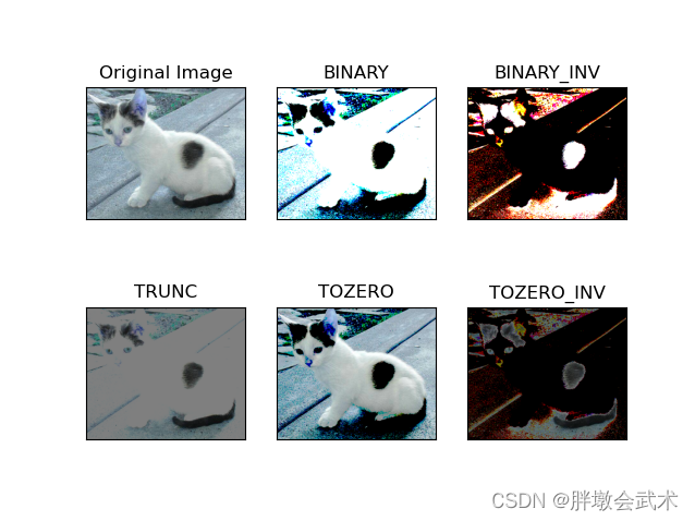
(七)阈值处理 —— cv2.threshold()
import cv2
import matplotlib.pyplot as plt
"""#############################################################
图像阈值 ret, dst = cv2.threshold(src, thresh, max_val, type)
输入参数        dst:    输出图
                src:    输入图,只能输入单通道图像,通常来说为灰度图
                thresh:     阈值
                max_val:    当像素值超过了阈值(或者小于阈值,根据type来决定),所赋予的值
                type:       二值化操作的类型,包含以下5种类型:
                    (1) cv2.THRESH_BINARY             超过阈值部分取max_val(最大值),否则取0
                  (2) cv2.THRESH_BINARY_INV         THRESH_BINARY的反转
                    (3) cv2.THRESH_TRUNC              大于阈值部分设为阈值,否则不变
                    (4) cv2.THRESH_TOZERO             大于阈值部分不改变,否则设为0
                    (5) cv2.THRESH_TOZERO_INV         THRESH_TOZERO的反转
#############################################################"""
img_BGR = cv2.imread(r'picture/cat.jpg')
ret, thresh1 = cv2.threshold(img_BGR, 127, 255, cv2.THRESH_BINARY)
ret, thresh2 = cv2.threshold(img_BGR, 127, 255, cv2.THRESH_BINARY_INV)
ret, thresh3 = cv2.threshold(img_BGR, 127, 255, cv2.THRESH_TRUNC)
ret, thresh4 = cv2.threshold(img_BGR, 127, 255, cv2.THRESH_TOZERO)
ret, thresh5 = cv2.threshold(img_BGR, 127, 255, cv2.THRESH_TOZERO_INV)

titles = ['Original Image', 'BINARY', 'BINARY_INV', 'TRUNC', 'TOZERO', 'TOZERO_INV']
images = [img_BGR, thresh1, thresh2, thresh3, thresh4, thresh5]

for ii in range(6):
    plt.subplot(2, 3, ii + 1), plt.imshow(images[ii], 'gray')
    plt.title(titles[ii])
    plt.xticks([]), plt.yticks([])
plt.show()
(八)均值/高斯/方框/中值滤波 —— cv2.blur() + cv2.boxFilter() + cv2.GaussianBlur() + cv2.medianBlur()

import cv2
import matplotlib.pyplot as plt
import numpy as np

img = cv2.imread(r'picture/cat.jpg')
"""######################################
均值滤波:cv2.blur(img, ksize) ———— 取卷积核所有元素的均值
输入参数      ksize 表示卷积核大小。   例如:(3, 3)
作用:对于椒盐噪声的滤除效果比较好。
######################################"""
blur = cv2.blur(img, (3, 3))

"""######################################
方框滤波:cv2.boxFilter(img, -1, (3, 3), normalize=True)
输入参数      normalize=True    选择归一化       即取所有元素之和除以卷积核大小(与均值滤波等同)
            normalize=False   不选择归一化     【容易越界】且当"元素之和>255",则等于255;
######################################"""
box_T = cv2.boxFilter(img, -1, (3, 3), normalize=True)
box_F = cv2.boxFilter(img, -1, (3, 3), normalize=False)

"""######################################
高斯滤波:cv2.GaussianBlur()
特点:高斯模糊的卷积核里的数值是满足高斯分布,相当于更重视中间的
######################################"""
aussian = cv2.GaussianBlur(img, (5, 5), 1)

"""######################################
中值滤波:cv2.medianBlur() ———— 取卷积核所有元素(从小到大排序)的中间值
作用:中值滤波对消除椒盐噪声非常有效,能够克服线性滤波器带来的图像细节模糊等弊端,能够有效保护图像边缘信息;
######################################"""
median = cv2.medianBlur(img, 5)

plt.subplot(2, 3, 1),    plt.imshow(img),        plt.title('raw')
plt.subplot(2, 3, 2),    plt.imshow(blur),       plt.title('blur')
plt.subplot(2, 3, 3),    plt.imshow(box_T),      plt.title('box_T')
plt.subplot(2, 3, 4),    plt.imshow(box_F),      plt.title('box_F')
plt.subplot(2, 3, 5),    plt.imshow(aussian),    plt.title('aussian')
plt.subplot(2, 3, 6),    plt.imshow(median),     plt.title('median')
plt.show()
"""######################################
np.hstack(img1, img2, img3)     在水平方向上平铺
np.vstack(img1, img2, img3)     在竖直方向上堆叠
######################################"""
res = np.hstack((blur, aussian, median))
cv2.imshow('median - Gaussian - average', res)
cv2.waitKey(0)
cv2.destroyAllWindows()

res = np.vstack((blur, aussian, median))
cv2.imshow('median - Gaussian - average', res)
cv2.waitKey(0)
cv2.destroyAllWindows()
(九)腐蚀与膨胀 —— cv2.erode() 与 cv2.dilate() + np.zeros() 与 np.ones()

import cv2
import numpy as np
import matplotlib.pyplot as plt
"""###########################################################
腐蚀操作:cv2.erode(src, kernel, iteration)
膨胀操作:cv2.dilate(src, kernel, iteration)
两者参数说明相同: src表示输入的图片, kernel表示方框的大小, iteration表示迭代的次数
###########################################################"""
img = cv2.imread(r'picture/dige.png')
kernel = np.ones((3, 3), np.uint8)

dilate_1 = cv2.dilate(img, kernel, iterations=1)
dilate_2 = cv2.dilate(img, kernel, iterations=2)
dilate_3 = cv2.dilate(img, kernel, iterations=3)

erosion_1 = cv2.erode(img, kernel, iterations=1)
erosion_2 = cv2.erode(img, kernel, iterations=2)
erosion_3 = cv2.erode(img, kernel, iterations=3)

plt.subplot(2, 3, 1),    plt.imshow(dilate_1),       plt.title('erode-1')
plt.subplot(2, 3, 2),    plt.imshow(dilate_2),       plt.title('erode-2')
plt.subplot(2, 3, 3),    plt.imshow(dilate_3),       plt.title('erode-3')
plt.subplot(2, 3, 4),    plt.imshow(erosion_1),      plt.title('dilate-1')
plt.subplot(2, 3, 5),    plt.imshow(erosion_2),      plt.title('dilate-2')
plt.subplot(2, 3, 6),    plt.imshow(erosion_3),      plt.title('dilate-3')
plt.show()
"""###########################################################
np.zeros()与np.ones():分别创建全0与全1的数组 —— 需导入numpy模块
两者输入参数相同,创建数组的方式也相同。
下面以np.zeros()为例
np.zeros(shape, dtype=float, order='C')
输入参数        (1)shape:生成numpy数组
            (2)dtype:指定生成的数据类型数据类型,可选参数
            (3)order:表示在内存中是以行为主存储还是以列为主存储,可选参数,c代表行优先(默认);F代表列优先
    创建一维数组:                      np.zeros(5)
    创建多维数组:                      np.zeros((5,2))
    创建int类型的数组:                 np.zeros((5,2),dtype=int)
    创建x为int类型,y为float类型的数组:np.zeros((5,2),dtype=[('x','int'),('y','float')]
###########################################################"""
(十)形态学变化 —— cv2.morphologyEx()
主要内容:开运算 + 闭运算 + 梯度计算 + 顶帽 + 黑帽

import cv2
import numpy as np
import matplotlib.pyplot as plt
"""#######################################
morphology
n. (生物)形态学;(语言学中的)词法,形态学;结构,形态
#######################################
morph
n. 形素,语素;形态;图像变换
v. (使)图像变形;将(图像)进行合成处理;改变,变化,变形
#######################################
形态学变化函数:cv2.morphologyEx(src, op, kernel)
参数说明:src传入的图片,op进行变化的方式, kernel表示方框的大小
op变化的方式有五种:
        开运算(open):             cv2.MORPH_OPEN              先腐蚀,再膨胀。                  开运算可以用来消除小黑点。
        闭运算(close):            cv2.MORPH_CLOSE             先膨胀,再腐蚀。                  闭运算可以用来突出边缘特征。
        形态学梯度(morph-grad):   cv2.MORPH_GRADIENT          膨胀后图像(减去)腐蚀图像。      可以突出团块(blob)的边缘,保留物体的边缘轮廓。
        顶帽(top-hat):            cv2.MORPH_TOPHAT            原始输入(减去)开运算结果。      将突出比原轮廓亮的部分。
        黑帽(black-hat):          cv2.MORPH_BLACKHAT          闭运算结果(减去)原始输入        将突出比原轮廓暗的部分。
#######################################"""
img = cv2.imread(r'picture/dige.png')
kernel = np.ones((5, 5), np.uint8)

img_open = cv2.morphologyEx(img, cv2.MORPH_OPEN, kernel)
img_close = cv2.morphologyEx(img, cv2.MORPH_CLOSE, kernel)
img_grad = cv2.morphologyEx(img, cv2.MORPH_GRADIENT, kernel)
img_top = cv2.morphologyEx(img, cv2.MORPH_TOPHAT, kernel)
img_black = cv2.morphologyEx(img, cv2.MORPH_BLACKHAT, kernel)

plt.subplot(2, 3, 1),    plt.imshow(img),            plt.title('RAW')
plt.subplot(2, 3, 2),    plt.imshow(img_open),       plt.title('MORPH_OPEN')
plt.subplot(2, 3, 3),    plt.imshow(img_close),      plt.title('MORPH_CLOSE')
plt.subplot(2, 3, 4),    plt.imshow(img_grad),       plt.title('MORPH_GRADIENT')
plt.subplot(2, 3, 5),    plt.imshow(img_top),        plt.title('MORPH_TOPHAT')
plt.subplot(2, 3, 6),    plt.imshow(img_black),      plt.title('MORPH_BLACKHAT')
plt.show()
(十一)边缘检测算子 —— cv2.sobel()、cv2.Scharr()、cv2.Laplacian()、cv2.Canny()
(1) 不同算子的差异:Sobel算子、Scharr算子、Laplacian算子
(2) Canny 不同阈值的区别

import cv2
import matplotlib.pyplot as plt
import numpy as np

img = cv2.imread(r'picture\lena.jpg')

sobel_Gx = cv2.Sobel(img, cv2.CV_64F, 1, 0, ksize=3)
sobel_Gx_Abs = cv2.convertScaleAbs(sobel_Gx)

sobel_Gy = cv2.Sobel(img, cv2.CV_64F, 0, 1, ksize=3)
sobel_Gy_Abs = cv2.convertScaleAbs(sobel_Gy)

sobel_Gx_Gy_Abs = cv2.addWeighted(sobel_Gx_Abs, 0.5, sobel_Gy_Abs, 0.5, 0)

plt.subplot(2, 3, 1),    plt.imshow(img),               plt.title('RAW')
plt.subplot(2, 3, 2),    plt.imshow(sobel_Gx),          plt.title('sobel_Gx')
plt.subplot(2, 3, 3),    plt.imshow(sobel_Gx_Abs),      plt.title('sobel_Gx_Abs')
plt.subplot(2, 3, 4),    plt.imshow(sobel_Gy),          plt.title('sobel_Gy')
plt.subplot(2, 3, 5),    plt.imshow(sobel_Gy_Abs),      plt.title('sobel_Gy_Abs')
plt.subplot(2, 3, 6),    plt.imshow(sobel_Gx_Gy_Abs),   plt.title('sobel_Gx_Gy_Abs')
plt.show()

"""########################################
Sobel算子: 是一种常用的边缘检测算子。对噪声具有平滑作用,提供较为精确的边缘方向信息,但是边缘定位精度不够高。
Sobel算子: 是离散微分算子(discrete differentiation operator),它结合了高斯平滑和微分求导,用来计算图像灰度的近似梯度,梯度越大越有可能是边缘。
        边缘就是像素对应的灰度值快速变化的地方。如:黑到白的边界
        图像是二维的。Sobel算子在x,y两个方向求导,故有不同的两个卷积核(Gx, Gy),且Gx的转置等于Gy。分别反映了每一点像素在水平方向和在垂直方向上的亮度变换情况.

########################################
dst = cv2.Sobel(src, ddepth, dx, dy, ksize)
输入参数    src        输入图像
          ddepth     图像的深度,-1表示采用的是与原图像相同的深度。目标图像的深度必须大于等于原图像的深度;
          dx和dy     表示的是求导的阶数,0表示这个方向上没有求导,一般为0、1、2。
          ksize      卷积核大小,一般为3、5。
同时对x和y进行求导,会导致部分信息丢失。(不建议)- 分别计算x和y,再求和(效果好)
########################################
(1)cv2.CV_16S的说明
      (1)Sobel函数求完导数后会有负值,还有会大于255的值。
      (2)而原图像是uint8,即8位无符号数。所以Sobel建立图像的位数不够,会有截断。
      (3)因此要使用16位有符号的数据类型,即cv2.CV_16S。
(2)cv2.convertScaleAbs(): 给图像的所有像素加一个绝对值
      通过该函数将其转回原来的uint8形式。否则将无法显示图像,而只是一副灰色的窗口。
############################################################################################"""

img = cv2.imread(r'picture\lena.jpg', cv2.IMREAD_GRAYSCALE)
sobelx = cv2.Sobel(img, cv2.CV_64F, 1, 0, ksize=3)
sobely = cv2.Sobel(img, cv2.CV_64F, 0, 1, ksize=3)
sobelx = cv2.convertScaleAbs(sobelx)
sobely = cv2.convertScaleAbs(sobely)
sobelxy = cv2.addWeighted(sobelx,0.5,sobely,0.5,0)

scharrx = cv2.Scharr(img, cv2.CV_64F, 1, 0)
scharry = cv2.Scharr(img, cv2.CV_64F, 0, 1)
scharrx = cv2.convertScaleAbs(scharrx)
scharry = cv2.convertScaleAbs(scharry)
scharrxy = cv2.addWeighted(scharrx, 0.5, scharry, 0.5, 0)

laplacian = cv2.Laplacian(img, cv2.CV_64F)
laplacian = cv2.convertScaleAbs(laplacian)

res = np.hstack((sobelxy, scharrxy, laplacian))
cv2.imshow('Sobel, Scharr, Laplacian', res)
cv2.waitKey(0)
cv2.destroyAllWindows()

"""############################################################################################
边缘检测Canny算子
(1)使用高斯滤波器,以平滑图像,滤除噪声。
(2)计算图像中每个像素点的梯度强度和方向。
(3)应用非极大值(Non-Maximum Suppression)抑制,以消除边缘检测带来的杂散响应。保留大值,去除小值。
(4)应用双阈值(Double-Threshold)检测来确定真实的和潜在的边缘。
(5)通过抑制孤立的弱边缘最终完成边缘检测。
############################################################################################"""
img = cv2.imread(r'picture\lena.jpg', cv2.IMREAD_GRAYSCALE)
v1 = cv2.Canny(img, 80, 150)
v2 = cv2.Canny(img, 50, 100)

res = np.hstack((v1, v2))
cv2.imshow('Canny', res)
cv2.waitKey(0)
cv2.destroyAllWindows()
(十二)图像金字塔 —— cv2.pyrUp()、cv2.pyrDown()

import cv2
import matplotlib.pyplot as plt

img = cv2.imread(r'picture\AM.png')
img_up = cv2.pyrUp(img)
img_up2 = cv2.pyrUp(img_up)

img_down = cv2.pyrDown(img)
img_down2 = cv2.pyrDown(img_down)

img_up_down = cv2.pyrDown(img_up)
img_down_up = cv2.pyrUp(img_down)

img_laplacian = img - img_down_up
plt.subplot(2, 4, 1),    plt.imshow(img),               plt.title('RAW')
plt.subplot(2, 4, 2),    plt.imshow(img_up),            plt.title('img_up')
plt.subplot(2, 4, 3),    plt.imshow(img_up2),           plt.title('img_up2')
plt.subplot(2, 4, 4),    plt.imshow(img_down),          plt.title('img_down')
plt.subplot(2, 4, 5),    plt.imshow(img_down2),         plt.title('img_down2')
plt.subplot(2, 4, 6),    plt.imshow(img_up_down),       plt.title('img_up_down')
plt.subplot(2, 4, 7),    plt.imshow(img_down_up),       plt.title('img_down_up')
plt.subplot(2, 4, 8),    plt.imshow(img_laplacian),     plt.title('img_laplacian')
plt.show()

"""############################################################################################
高斯金字塔: cv2.pyrUp 与 cv2.pyrDown
  cv2.pyrDown:  向下采样(缩小一倍)。          (1)对图像进行高斯内核卷积;(2)将所有偶数行和列去除;
  cv2.pyrUp:    向上采样(放大一倍),分辨率降低。(1)将图像每隔"一行与一列",全部填充0;(2)使用先前同样的高斯内核(乘以4)与放大后的图像卷积,获得近似值;
形成过程大致:     (1)对原图像进行低通滤波和降采样得到一个粗尺度的近似图像,即分解得到的低通近似图像,
                (2)对近似图像经过插值(即上采样)和低通滤波
                (3)计算它和原图像的差值,得到分解的带通分量。
                ——— 第一步:源图像先缩小后再放大; 第二步:源图像减去第一步操作后得到新图像。
图像缩放: (1)图像金字塔(2)resize()函数; 后者效果更好,不会降低分辨率。
############################################################################################"""
(十三)图像轮廓检测 —— cv2.findContours()、cv2.drawContours()、cv2.arcLength()、cv2.approxPolyDP()、cv2.rectangle()
(1) 轮廓的多边形拟合曲线:cv2.approxPolyDP()
(2) 用矩形画出轮廓的边界:cv2.boundingRect()、cv2.rectangle()
(3) 用外接圆画出轮廓的边界:cv2.minEnclosingCircle()、cv2.circle()

import cv2
import matplotlib.pyplot as plt

img = cv2.imread(r'picture\contours2.png')
img_gray = cv2.cvtColor(img, cv2.COLOR_BGR2GRAY)
ret, thresh = cv2.threshold(img_gray, 127, 255, cv2.THRESH_BINARY)

draw_img1 = img.copy()
contours, hierarchy = cv2.findContours(thresh, cv2.RETR_TREE, cv2.CHAIN_APPROX_NONE)

res1 = cv2.drawContours(draw_img1, contours, -1, (0, 0, 255), 2)

draw_img2 = img.copy()
contours1 = contours[0]
epsilon = 0.21*cv2.arcLength(contours1, True)
approx = cv2.approxPolyDP(contours1, epsilon, True)

res2 = cv2.drawContours(draw_img2, [approx], -1, (0, 0, 255), 2)

draw_img3 = img.copy()
x, y, w, h = cv2.boundingRect(contours1)
img_rectangle = cv2.rectangle(draw_img3, (x, y), (x+w, y+h), (0, 255, 0), 2)

draw_img4 = img.copy()
(x, y), radius = cv2.minEnclosingCircle(contours1)
center = (int(x), int(y))
radius = int(radius)
img_circle = cv2.circle(draw_img4, center, radius, (0, 255, 0), 2)

plt.subplot(2, 3, 1),    plt.imshow(img),               plt.title('RAW')
plt.subplot(2, 3, 2),    plt.imshow(res1),              plt.title('findContours')
plt.subplot(2, 3, 3),    plt.imshow(res2),              plt.title('approxPolyDP')
plt.subplot(2, 3, 4),    plt.imshow(draw_img3),         plt.title('rectangle')
plt.subplot(2, 3, 5),    plt.imshow(draw_img4),         plt.title('circle')
plt.show()

"""######################################################################
(1)轮廓检测:contours, hierarchy = cv2.findContours(img, mode, method)
输入参数      mode: 轮廓检索模式
                  (1)RETR_EXTERNAL:  只检索最外面的轮廓;
                  (2)RETR_LIST:      检索所有的轮廓,但检测的轮廓不建立等级关系,将其保存到一条链表当中,
                  (3)RETR_CCOMP:     检索所有的轮廓,并建立两个等级的轮廓。顶层是各部分的外部边界,内层是的边界信息;
                  (4)RETR_TREE:      检索所有的轮廓,并建立一个等级树结构的轮廓;(最常用)
              method: 轮廓逼近方法
                  (1)CHAIN_APPROX_NONE:      存储所有的轮廓点,相邻的两个点的像素位置差不超过1。               例如:矩阵的四条边。(最常用)
                  (2)CHAIN_APPROX_SIMPLE:     压缩水平方向,垂直方向,对角线方向的元素,只保留该方向的终点坐标。   例如:矩形的4个轮廓点。
输出参数      contours:所有的轮廓
              hierarchy:每条轮廓对应的属性
备注0:轮廓就是将连续的点(连着边界)连在一起的曲线,具有相同的颜色或者灰度。轮廓在形状分析和物体的检测和识别中很有用。
备注1:函数输入图像是二值图,即黑白的(不是灰度图)。所以读取的图像要先转成灰度的,再转成二值图。
备注2:函数在opencv2只返回两个值:contours, hierarchy。
备注3:函数在opencv3会返回三个值:img, countours, hierarchy
######################################################################
(2)绘制轮廓:v2.drawContours(image, contours, contourIdx, color, thickness) ———— (在图像上)画出图像的轮廓
输入参数        image:              需要绘制轮廓的目标图像,注意会改变原图
                contours:           轮廓点,上述函数cv2.findContours()的第一个返回值
                contourIdx:         轮廓的索引,表示绘制第几个轮廓。-1表示绘制所有的轮廓
                color:              绘制轮廓的颜色(RGB)
                thickness:          (可选参数)轮廓线的宽度,-1表示填充
备注:图像需要先复制一份copy(), 否则(赋值操作的图像)与原图会随之一起改变。
######################################################################
(3)计算轮廓的长度:retval = cv2.arcLength(curve, closed)
输入参数:      curve              轮廓(曲线)。
                closed             若为true,表示轮廓是封闭的;若为false,则表示打开的。(布尔类型)
#
输出参数:      retval             轮廓的长度(周长)。
######################################################################
(4)找出轮廓的多边形拟合曲线:approxCurve = approxPolyDP(contourMat, epsilon, closed);
输入参数:     contourMat:        轮廓点矩阵(集合)
               epsilon:           (double类型)指定的精度, 即原始曲线与近似曲线之间的最大距离。
               closed:            (bool类型)若为true, 则说明近似曲线是闭合的; 反之, 若为false, 则断开。
#
输出参数:     approxCurve:       轮廓点矩阵(集合);当前点集是能最小包容指定点集的。画出来即是一个多边形;
######################################################################
(5)绘制矩形边框:cv2.rectangle(img, (x, y), (x+w, y+h), (0, 255, 0), 2)
      (x, y):         矩形定点
      (x+w, y+h):     矩形的宽高
      (0,0,225):      矩形的边框颜色;
      2:              矩形边框宽度
######################################################################"""
(十四)模板匹配 —— cv2.matchTemplate()、cv2.minMaxLoc()

import cv2
import matplotlib.pyplot as plt

img = cv2.imread(r'picture/lena.jpg', 0)
template = cv2.imread(r'picture/face.jpg', 0)
h, w = template.shape[::1]

res1 = cv2.matchTemplate(img, template, cv2.TM_SQDIFF)
min_val1, max_val1, min_loc1, max_loc1 = cv2.minMaxLoc(res1)
top_left1 = min_loc1
bottom_right1 = (top_left1[0] + w, top_left1[1] + h)

res2 = cv2.matchTemplate(img, template, cv2.TM_CCORR)
min_val2, max_val2, min_loc2, max_loc2 = cv2.minMaxLoc(res2)
top_left2 = max_loc2
bottom_right2 = (top_left2[0] + w, top_left2[1] + h)

res3 = cv2.matchTemplate(img, template, cv2.TM_CCOEFF)
min_val3, max_val3, min_loc3, max_loc3 = cv2.minMaxLoc(res3)
top_left3 = max_loc3
bottom_right3 = (top_left3[0] + w, top_left3[1] + h)

res4 = cv2.matchTemplate(img, template, cv2.TM_SQDIFF_NORMED)
min_val4, max_val4, min_loc4, max_loc4 = cv2.minMaxLoc(res4)
top_left4 = min_loc4
bottom_right4 = (top_left4[0] + w, top_left4[1] + h)

res5 = cv2.matchTemplate(img, template, cv2.TM_CCORR_NORMED)
min_val5, max_val5, min_loc5, max_loc5 = cv2.minMaxLoc(res5)
top_left5 = max_loc5
bottom_right5 = (top_left5[0] + w, top_left5[1] + h)

res6 = cv2.matchTemplate(img, template, cv2.TM_CCOEFF_NORMED)
min_val6, max_val6, min_loc6, max_loc6 = cv2.minMaxLoc(res6)
top_left6 = max_loc6
bottom_right6 = (top_left6[0] + w, top_left6[1] + h)

img1 = img.copy();       img2 = img.copy();           img3 = img.copy()
img4 = img.copy();       img5 = img.copy();           img6 = img.copy()

cv2.rectangle(img1, top_left1, bottom_right1, 255, 2)
cv2.rectangle(img2, top_left2, bottom_right2, 255, 2)
cv2.rectangle(img3, top_left3, bottom_right3, 255, 2)
cv2.rectangle(img4, top_left4, bottom_right4, 255, 2)
cv2.rectangle(img5, top_left5, bottom_right5, 255, 2)
cv2.rectangle(img6, top_left6, bottom_right6, 255, 2)

plt.subplot(231),       plt.imshow(img1, cmap='gray'),         plt.axis('off'),        plt.title('cv2.TM_SQDIFF')
plt.subplot(232),       plt.imshow(img2, cmap='gray'),         plt.axis('off'),        plt.title('cv2.TM_CCORR')
plt.subplot(233),       plt.imshow(img3, cmap='gray'),         plt.axis('off'),        plt.title('cv2.TM_CCOEFF')
plt.subplot(234),       plt.imshow(img4, cmap='gray'),         plt.axis('off'),        plt.title('cv2.TM_SQDIFF_NORMED')
plt.subplot(235),       plt.imshow(img5, cmap='gray'),         plt.axis('off'),        plt.title('cv2.TM_CCORR_NORMED')
plt.subplot(236),       plt.imshow(img6, cmap='gray'),         plt.axis('off'),        plt.title('cv2.TM_CCOEFF_NORMED')
plt.show()
"""##############################################
模板匹配:cv2.matchTemplate(image, template, method)
输入图像:检测对象的图像
模板图像:待检测的对象特征
模板匹配方法:
          (1)cv2.TM_SQDIFF:         计算平方差。           计算出来的值越接近0,越相关
          (2)cv2.TM_CCORR:          计算相关性。           计算出来的值越大,越相关
          (3)cv2.TM_CCOEFF:         计算相关系数。         计算出来的值越大,越相关
          (4)cv2.TM_SQDIFF_NORMED:  计算(归一化)平方差。   计算出来的值越接近0,越相关
          (5)cv2.TM_CCORR_NORMED:   计算(归一化)相关性。   计算出来的值越接近1,越相关
          (6)cv2.TM_CCOEFF_NORMED:  计算(归一化)相关系数。  计算出来的值越接近1,越相关
(最好选择有归一化操作,效果好)
##############################################
获取匹配结果函数:min_val, max_val, min_loc, max_loc = cv2.minMaxLoc(ret)
其中: ret是cv2.matchTemplate函数返回的矩阵;
      min_val, max_val, min_loc, max_loc分别表示最小值,最大值,最小值与最大值在图像中的位置
如果模板方法是平方差或者归一化平方差,要用min_loc; 其余用max_loc
##############################################"""
(十五)直方图(均衡化) —— cv2.calcHist()、img.ravel()、cv2.bitwise_and()、cv2.equalizeHist()、cv2.createCLAHE()
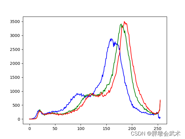

import cv2
import matplotlib.pyplot as plt
import numpy as np

img = cv2.imread(r'picture\cat.jpg', 0)
hist = cv2.calcHist([img], [0], None, [256], [0, 256])
plt.hist(img.ravel(), 256)
plt.show()

img1 = cv2.imread(r'picture\cat.jpg', 1)
color = ('blue', 'green', 'red')
for i, col in enumerate(color):
    hist1 = cv2.calcHist([img1], [i], None, [256], [0, 256])
    plt.plot(hist1, color=col)
plt.show()
"""##############################################
统计每个像素的众数(备注:输入参数需用方括号[]表示)
直方图: cv2.calcHist(images,channels,mask,histSize,ranges)
输入参数:     images:          原图像图像格式必须为 uint8 或 float32。
             channels:        (1)灰度图:[0]; (2)彩色图像:[0] [1] [2],分别对应着BGR。
             mask:            掩模图像。(1)统计整幅图像的直方图,则设置为 None。(2)统计图像某一区域的直方图,则制作一个掩模图像。
             histSize:        BIN的数目。可以理解为迭代范围。如:[1]表示0,1,2...256;如[10]表示0~10,11~20...;如[256]表示0~256。
             ranges:          统计像素值范围。通常为[0~256]。

##############################################"""

mask = np.zeros(img.shape[:2], np.uint8)
mask[100:300, 100:400] = 255
masked_img = cv2.bitwise_and(img, img, mask=mask)
hist_full = cv2.calcHist([img], [0], None, [256], [0, 256])
hist_mask = cv2.calcHist([img], [0], mask, [256], [0, 256])
plt.subplot(221), plt.imshow(img, 'gray'),                  plt.title('Raw')
plt.subplot(222), plt.imshow(mask, 'gray'),                 plt.title('mask')
plt.subplot(223), plt.imshow(masked_img, 'gray'),           plt.title('cv2.bitwise_and')
plt.subplot(224), plt.plot(hist_full), plt.plot(hist_mask), plt.title('hist_full + hist_mask')
plt.subplot(224), plt.plot(hist_full), plt.plot(hist_mask), plt.title('hist_full + hist_mask')
plt.xlim([0, 256])
plt.show()

img = cv2.imread(r'picture\cat.jpg', 0)
equ = cv2.equalizeHist(img)

clahe = cv2.createCLAHE(clipLimit=2.0, tileGridSize=(8, 8))
res_clahe = clahe.apply(img)
plt.subplot(131),   plt.imshow(img, 'gray'),        plt.title('Raw')
plt.subplot(132),   plt.imshow(equ, 'gray'),        plt.title('cv2.equalizeHist')
plt.subplot(133),   plt.imshow(res_clahe, 'gray'),  plt.title('cv2.createCLAHE')
plt.show()
(十六)傅里叶变换 + 低通/高通滤波 —— cv2.dft()、cv2.idft()、np.fft.fftshift()、np.fft.ifftshift()、cv2.magnitud()
傅里叶变换
以时间作为参照来观察动态世界的方法我们称其为时域分析。
世间万物都在随着时间不停的改变,并且永远不会静止下来。但在频域中,你会发现世界是静止的、永恒不变的。
傅里叶告诉我们:任何周期函数,都可以看作是不同振幅,不同相位正弦波的叠加。
举例:利用对不同琴键不同力度,不同时间点的敲击,可以组合出任何一首乐曲。
傅里叶分析可分为傅里叶级数(Fourier Serie)和傅里叶变换(Fourier Transformation)。
傅里叶变换的作用
(1)高频:变化剧烈的灰度分量,例如:边界/图像的轮廓
(2)低频:变化缓慢的灰度分量,例如:一片大海
滤波器
(1)低通滤波器:只保留低频,会使得图像模糊

"""##############################################
傅里叶变换:cv2.dft(np.float32, cv2.DFT_COMPLEX_OUTPUT)
输入参数:  (1)输入图像需要先转换成np.float32 格式。
          (2)转换标识 - cv2.DFT_COMPLEX_OUTPUT - 用来输出一个复数阵列
逆傅里叶变换:cv2.idft(dft_shift)
输入参数:  (1)傅里叶变换后并位置转换后的频谱图像。

在OpenCV中,我们通过cv2.dft()来实现傅里叶变换,使用cv2.idft()来实现逆傅里叶变换。
    注意1:变换后得到原始图像的频谱信息。其中:频率为0的部分(零分量)会在左上角,需要使用numpy.fft.fftshift()函数,将其移动到中间位置。
    注意2:变换后的频谱图像是双通道的(实部,虚部)。需要使用cv2.magnitude函数,将幅度映射到灰度空间[0,255]内,使其以灰度图像显示出来。

cv2.magnitude(x-实部,y-虚部)
输入参数:   (1)浮点型x坐标值(实部)
           (2)浮点型y坐标值(虚部)
备注:两个参数的必须具有相同的大小(size)
##############################################"""

img = cv2.imread(r'picture\lena.jpg', 0)
dft = cv2.dft(np.float32(img), flags=cv2.DFT_COMPLEX_OUTPUT)
dft_shift = np.fft.fftshift(dft)
magnitude_spectrum = 20*np.log(cv2.magnitude(dft_shift[:, :, 0],dft_shift[:, :, 1]))

rows, cols = img.shape
crow, ccol = int(rows/2), int(cols/2)

mask_low = np.zeros((rows, cols, 2), np.uint8)
mask_low[crow-30:crow+30, ccol-30:ccol+30] = 1

fshift_low = dft_shift * mask_low
f_ishift_low = np.fft.ifftshift(fshift_low)
img_low = cv2.idft(f_ishift_low)
img_low = cv2.magnitude(img_low[:, :, 0], img_low[:, :, 1])

mask_high = np.ones((rows, cols, 2), np.uint8)
mask_high[crow-30:crow+30, ccol-30:ccol+30] = 0

fshift_high = dft_shift * mask_high
f_ishift_high = np.fft.ifftshift(fshift_high)
img_high = cv2.idft(f_ishift_high)
img_high = cv2.magnitude(img_high[:, :, 0], img_high[:, :, 1])

plt.subplot(141),  plt.imshow(img, cmap='gray'),                 plt.title('Input Image'),        plt.xticks([]),   plt.yticks([])
plt.subplot(142),  plt.imshow(magnitude_spectrum, cmap='gray'),  plt.title('Magnitude Spectrum'), plt.xticks([]),   plt.yticks([])
plt.subplot(143),  plt.imshow(img_low, cmap='gray'),   plt.title('Low pass filter'),   plt.xticks([]),   plt.yticks([])
plt.subplot(144),  plt.imshow(img_high, cmap='gray'),  plt.title('High pass filter'),  plt.xticks([]),   plt.yticks([])
plt.show()
(十七)Harris角点检测 —— cv2.cornerHarris()、np.float32()

import cv2
import numpy as np

img = cv2.imread(r'picture\Black_and_white_chess.jpg')
print('img.shape:', img.shape)

gray = cv2.cvtColor(img, cv2.COLOR_BGR2GRAY)
gray = np.float32(gray)
"""#################################################
Harris角点检测:res = cv2.cornerHarris(img_gray, blockSize, k_size, k)
输入参数       img_gray       数据类型为 float32 的输入图像。
              blockSize      角点检测中要考虑的领域大小        (一般等于2)
              k_size         Sobel求导中使用的窗口大小        (一般等于3)
              k              方程中检测器的自由参数, 取值参数为 [0,04,0.06].

角点定义: 角点是一个无论框框往哪边移动 框框内像素值都会变化很大的情况而定下来的点。
##################################################
float16 半精度浮点数,包括:1 个符号位,5 个指数位,10 个尾数位
float32 单精度浮点数,包括:1 个符号位,8 个指数位,23 个尾数位
float64 双精度浮点数,包括:1 个符号位,11 个指数位,52 个尾数位
##################################################"""
Harris_dst = cv2.cornerHarris(gray, 2, 3, 0.04)
print('dst.shape:', Harris_dst.shape)

img[Harris_dst > 0.01 * Harris_dst.max()] = [0, 0, 255]

cv2.imshow('Harris_dst', img)
cv2.waitKey(0)
cv2.destroyAllWindows()
(十八)SIFT尺度不变特征检测 —— cv2.xfeatures2d.SIFT_create()、sift.detectAndCompute()、sift.detect()、sift.compute()、cv2.drawKeypoints

"""#########################################################
SIFT 图像特征检测算法
(Scale-invariant feature transform,SIFT)尺度不变特征变换。
特点:具有尺度不变性。即对图片进行放缩、变形、模糊、明暗变化、光照变化、添加噪声,甚至是使用不同的相机拍摄不同角度的照片的情况下,SIFT都能检测到稳定的特征点,并建立对应关系。
缺点:计算量比较大,很难实时
对比:Harris角点检测算法最大的缺陷是不具有尺度不变性。当图片放大后,原来能检测到的角点就变成了边线,就检测不到了
#########################################################
在Opencv中,SIFT函数从3.4.3版本以上已经涉及到专利保护。顾Opencv需要降版本使用。
卸载旧版本:pip uninstall opencv-python
          pip uninstall opencv-contrib-python
安装新版本:pip install opencv-python==3.4.1.15
          pip install opencv-contrib-python==3.4.1.15
#########################################################"""
import cv2

img = cv2.imread('test_1.jpg')
gray = cv2.cvtColor(img, cv2.COLOR_BGR2GRAY)

sift = cv2.xfeatures2d.SIFT_create()
"""#########################################################
检测关键点并计算描述子:key_points, des = sift.detectAndCompute(img, None)
输出参数:key_points为图像关键点;dst为sift特征向量,通常是128维。
#
其中,sift.detectAndCompute()可以拆分为以下两个函数:sift.detect()和sift.compute()。
      key_points = sift.detect(gray, None)         # 找出图像中的关键点
      kp, dst = sift.compute(key_points)           # 计算关键点对应的sift特征向量
#########################################################"""
key_points, des = sift.detectAndCompute(gray, None)

"""#########################################################
在图中画出关键点:ret = cv2.drawKeypoints(gray, key_points, img)
输入参数:gray表示输入图片;kp表示关键点;img表示输出的图片
#########################################################"""
img = cv2.drawKeypoints(gray, key_points, img)

cv2.imshow('key_points', img)
cv2.waitKey(0)
cv2.destroyAllWindows()
(十九)暴力特征匹配 —— cv2.BFMatcher_create()、bf.match()、bf_knn.knnMatch()、cv2.drawMatches()

"""########################################################
暴力特征检测主要流程
              (1)先在查询描述符中取一个关键点的描述符,将其与训练描述符中的所有关键点描述符进行比较。
              (2)每次比较后会计算出一个距离值,距离最小的值对应最佳匹配结果。
              (3)所有描述符比较完后,匹配器返回匹配结果列表。
########################################################
在Opencv中,SIFT函数从3.4.3版本以上已经涉及到专利保护。顾Opencv需要降版本使用。
卸载旧版本:pip uninstall opencv-python
          pip uninstall opencv-contrib-python
安装新版本:pip install opencv-python==3.4.1.15
          pip install opencv-contrib-python==3.4.1.15
########################################################"""
import cv2
import matplotlib.pyplot as plt

img1 = cv2.imread(r'picture\box.png')
img2 = cv2.imread(r'picture\box_in_scene.png')

sift = cv2.xfeatures2d.SIFT_create()

kp1, des1 = sift.detectAndCompute(img1, None)
kp2, des2 = sift.detectAndCompute(img2, None)

bf = cv2.BFMatcher_create(cv2.NORM_L1, crossCheck=False)
matches = bf.match(des1, des2)
matches = sorted(matches, key=lambda x: x.distance)
result = cv2.drawMatches(img1, kp1, img2, kp2, matches[:15], None)

bf_knn = cv2.BFMatcher_create(cv2.NORM_HAMMING, crossCheck=False)
ms_knn = bf_knn.knnMatch(des1, des2, k=2)

good = []
for m, n in ms_knn:
    if m.distance < 0.75 * n.distance:
        good.append(m)
img_DEFAUL = cv2.drawMatches(img1, kp1, img2, kp2, good[:20], None, flags=cv2.DrawMatchesFlags_DEFAUL)
img_NO_POINTS = cv2.drawMatches(img1, kp1, img2, kp2, good[:20], None, flags=cv2.DrawMatchesFlags_NOT_DRAW_SINGLE_POINTS)
img_KEYPOINTS = cv2.drawMatches(img1, kp1, img2, kp2, good[:20], None, flags=cv2.DrawMatchesFlags_DRAW_RICH_KEYPOINTS)

plt.subplot(231),       plt.imshow(img1),               plt.title('raw_img1')
plt.subplot(232),       plt.imshow(img2),               plt.title('raw_img2')
plt.subplot(233),       plt.imshow(result),             plt.title('match_result')

plt.subplot(234),       plt.imshow(img_DEFAUL),         plt.title('knnMatch_DEFAUL')
plt.subplot(235),       plt.imshow(img_NO_POINTS),      plt.title('knnMatch_NO_POINTS')
plt.subplot(236),       plt.imshow(img_KEYPOINTS),      plt.title('knnMatch_KEYPOINTS')
plt.show()
"""########################################################
暴力匹配器:bf = cv2.BFMatcher_create(normType, crossCheck)
输出参数          bf               返回的暴力匹配器对象
输入参数          crossCheck       默认为False, 表示匹配器为每个查询描述符找到k个距离最近的匹配描述符。若为True, 则只返回满足交叉验证条件的匹配结果。
                 normType         距离测量类型
                    方法(1)【SIFT】描述符使用cv2.NORM_L1或cv2.NORM_L2,默认为cv2.NORM_L2。
                    方法(2)【ORB】描述符使用cv2.NORM_HAMMING
###########################
(1)匹配最佳结果:ms = bf.match(des1, des2)
输出参数          ms          为每个关键点的最佳匹配结果(距离值越小匹配度越高)
输入参数          des1        为查询描述符
                 des2         为训练描述符
###########################
(2)匹配指定数量的最佳结果:ms = knnMatch(des1, des2, k=n)
输出参数          ms          为返回的匹配结果, 每个列表元素是一个子列表, 它包含了由参数k指定个数的DMatch对象
输入参数          des1        为查询描述符
                 des2       为训练描述符
                 k          为返回的最佳匹配个数
########################################################
绘制最佳匹配:outImg = cv2.drawMatches(img1, keypoints1, img2, keypoints2, matches1to2[, matchColor[, singlePointColor[, matchesMask[, flags]]]])
输出参数         outImg为返回的绘制结果图像, 图像中查询图像与训练图像中匹配的关键点个两点之间的连线为彩色
输入参数        (1)img1为查询图像               (2)keypoints1为img1的关键点
               (3)img2为训练图像               (4)keypoints2为img2的关键点
               (5)matches1to2         img1与img2的匹配结果
               (6)matchColor          关键点和链接线的颜色, 默认使用随机颜色
               (7)singlePointColor    单个关键点的颜色, 默认使用随机颜色
               (8)matchesMask         掩膜, 用于决定绘制哪些匹配结果, 默认为空, 表示绘制所有匹配结果
flags为标志, 可设置为下列参数值:
      (1)cv2.DrawMatchesFlags_DEFAUL                     (默认方式)绘制两个源图像、匹配项和单个关键点, 没有围绕关键点的圆以及关键点的大小和方向
      (2)cv2.DrawMatchesFlags_NOT_DRAW_SINGLE_POINTS     不会绘制单个关键点
      (3)cv2.DrawMatchesFlags_DRAW_RICH_KEYPOINTS        在关键点周围绘制具有关键点大小和方向的圆圈
########################################################"""
(二十)图像缩放+镜像+平移+旋转+仿射变换+透视变换 —— cv2.resize()、cv2.getRotationMatrix2D()、cv2.getAffineTransform()、cv2.getPerspectiveTransform()、cv2.warpPerspective()、cv2.warpAffine()

import cv2
import numpy as np
import matplotlib.pyplot as plt

img = cv2.imread(r"picture/1.jpg", 1)
imgInfo = img.shape
height = imgInfo[0]; width = imgInfo[1]; deep = imgInfo[2]

dstHeight = int(height/2)
dstWidth = int(width/2)
dst_resize_dir = cv2.resize(img, (dstWidth, dstHeight))

dst_resize_linear = np.zeros([dstHeight, dstWidth, 3], np.uint8)
for i in range(dstHeight):
    for j in range(dstWidth):
        iNew = i * (height * 1.0 / dstHeight)
        jNew = j * (width * 1.0 / dstWidth)
        dst_resize_linear[i, j] = img[int(iNew), int(jNew)]

dst_mirror = np.zeros([height * 2, width, deep], np.uint8)
for i in range(height):
    for j in range(width):
        dst_mirror[i, j] = img[i, j]
        dst_mirror[height * 2 - i - 1, j] = img[i, j]
for i in range(width):
    dst_mirror[height, i] = (0, 0, 255)

dst_trans = np.zeros(imgInfo, np.uint8)
for i in range(height):
    for j in range(width - 200):
        dst_trans[i, j+100] = img[i, j]

matRotate = cv2.getRotationMatrix2D((height*0.5, width*0.5), 45, 0.7)
dst_rotate = cv2.warpAffine(img, matRotate, (height, width))

matSrc = np.float32([[0, 0], [0, height-1], [width-1, 0]])
matDst = np.float32([[50, 50], [100, height-50], [width-200, 100]])
matAffine = cv2.getAffineTransform(matSrc, matDst)
dst_affine = cv2.warpAffine(img, matAffine, (height, width))

matDst1 = np.float32([[50, 50], [100, height-50], [width-200, 100], [width-200, height-50]])
matSrc1 = np.float32([[0, 0], [0, height-1], [width-1, 0], [width-1, height-1]])
matwarp = cv2.getPerspectiveTransform(matDst1, matSrc1)
dst_Perspective = cv2.warpPerspective(img, matwarp, (height, width))
dst_Perspective = np.hstack((dst_affine, dst_Perspective))

plt.subplot(241),       plt.imshow(img, 'gray'),                    plt.title('img')
plt.subplot(242),       plt.imshow(dst_resize_dir, 'gray'),         plt.title('dst_resize_dir (coordinates)')
plt.subplot(243),       plt.imshow(dst_resize_linear, 'gray'),      plt.title('dst_resize_linear (coordinates)')
plt.subplot(244),       plt.imshow(dst_mirror, 'gray'),             plt.title('dst_mirror')
plt.subplot(245),       plt.imshow(dst_trans, 'gray'),              plt.title('dst_trans')
plt.subplot(246),       plt.imshow(dst_rotate, 'gray'),             plt.title('dst_rotate')
plt.subplot(247),       plt.imshow(dst_affine, 'gray'),             plt.title('dst_affine')
plt.subplot(248),       plt.imshow(dst_Perspective, 'gray'),        plt.title('dst_Perspective')
plt.show()

"""################################################
图像缩小或放大:cv2.resize(src, dsize, fx=0, fy=0, interpolation=INTER_LINEAR)
输入参数:       src                输入图片
               dsize            (1)矩阵参数缩放到指定大小(width,height);           例如:cv2.resize(img_dog, (500, 414))
                                (2)矩阵参数为(0,0),原图像缩放倍数通过fx, fy来控制;    例如:cv2.resize(img_dog, (0, 0), fx=4, fy=4)
               fx, fy             沿x轴,y轴的缩放系数
               interpolation      插值方法,有以下五种(可选参数)
                          (1)INTER_NEAREST       最近邻插值                   (2)INTER_LINEAR        双线性插值(默认设置)
                          (3)INTER_AREA          使用像素区域关系进行重采样。     (4)INTER_CUBIC         4x4像素邻域的双三次插值
                          (5)INTER_LANCZOS4      8x8像素邻域的Lanczos插值
################################################
获取旋转矩阵:rot_mat = cv2.getRotationMatrix2D(center, angle, scale)
输入参数          center        旋转的中心点。一般是图像的中心,取图像长宽的一半
                angle         旋转的角度。正值是顺时针旋转,负值是逆时针旋转
                scale         缩放比例。
################################################
获取仿射变换矩阵:matAffine = cv2.getAffineTransform(matSrc, matDst)
输入参数        matSrc          原图的三个点坐标
              matDst          仿射的三个点坐标
输出参数        matAffine       仿射变换矩阵
################################################
计算齐次变换矩阵:cv2.getPerspectiveTransform(rect, dst)
输入参数        rect输入图像的四个点(四个角)
                dst输出图像的四个点(方方正正的图像对应的四个角)
################################################
仿射变换:cv2.warpPerspective(src, M, dsize, dst=None, flags=None, borderMode=None, borderValue=None)
透视变换:cv2.warpAffine(src, M, dsize, dst=None, flags=None, borderMode=None, borderValue=None)
                src:输入图像     dst:输出图像
                M:2×3的变换矩阵
                dsize:变换后输出图像尺寸
                flag:插值方法
                borderMode:边界像素外扩方式
                borderValue:边界像素插值,默认用0填充
#
(Affine Transformation)可实现旋转,平移,缩放,变换后的平行线依旧平行。
(Perspective Transformation)即以不同视角的同一物体,在像素坐标系中的变换,可保持直线不变形,但是平行线可能不再平行。
#
备注:cv2.warpAffine需要与cv2.getRotationMatrix2D/cv2.getAffineTransform/cv2.getPerspectiveTransform搭配使用。
################################################"""
Original: https://blog.csdn.net/shinuone/article/details/126022763
Author: 胖墩会武术
Title: Opencv图像处理(全)
原创文章受到原创版权保护。转载请注明出处:https://www.johngo689.com/705105/
转载文章受原作者版权保护。转载请注明原作者出处!