


CVPR-2021
文章目录
- 1 Background and Motivation
- 2 Related Work
- 3 Advantages / Contributions
- 4 Method
* - 4.1 Multistage processing pipeline
- 4.2 Refinement module
- 4.3 MagNetFast
- 5 Experiments
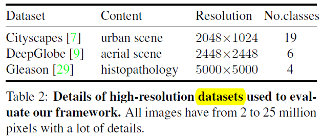
* - 5.1 Datasets
- 5.2 Experiments on the Cityscapes dataset
- 5.3 DeepGlobe
- 5.4 Gleason
- 6 Conclusion(own)
; 1 Background and Motivation
做高分辨率图像分割任务的时候,由于 GPU 资源的限制,不能直接训练原图
解决办法往往是 downsample the big image or divide the image into local patches for separate processing
然而 downsample 会丢失很多细节,patches 方法缺乏大局观(全局信息)
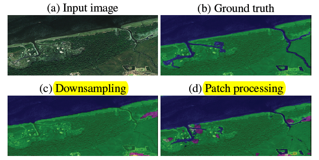
作者结合上述两种方法的优点,提出了 a multi-scale segmentation framework for high-resolution images——MagNet
在 Cityscapes / DeepGlobe / Gleason 三个高分辨率图片数据集上验证了其有效性
2 Related Work
- Multi-scale, eg:FPN / ASPP / HRNet
- multi-stage, eg:Auto-ZoomNet
- context aggregation,eg:BiseNet
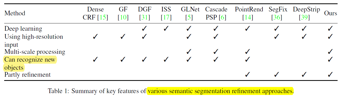
- Segmentation refinement
; 3 Advantages / Contributions
针对高分辨率图像分割问题,设计 MagNet 网络,Experiments on three high-resolution datasets of urban views, aerial scenes, and medical images show that MagNet consistently outperforms the state-of-theart methods by a significant margin
4 Method
核心模块有两个
- segmentation network(module,普通的分割网络)
- refinement module(作者提出的)
4.1 Multistage processing pipeline
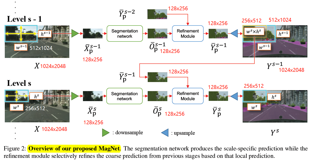
- s 表示 scale
- p 表示 patch
- X 表示输入图片
- Y 表示输出图片
- X ˉ \bar{X}X ˉ 表示输入到 segmentation network 中的 tensor,尺寸固定
- Y ˉ \bar{Y}Y ˉ 表示从 refinement module 中输出的 tensor,尺寸固定
- O ˉ \bar{O}O ˉ 表示从 segmentation network 中输出的 tensor,尺寸固定
以 4 scale 为例子
假如输入图片 h 和 w 为 1024×2048
各个 scale 下的 patch 的大小为:
1024×2048
512×1024
256×512
128×256
segmentation 和 refinement 模块的输入输出都为 128×256
; 4.2 Refinement module
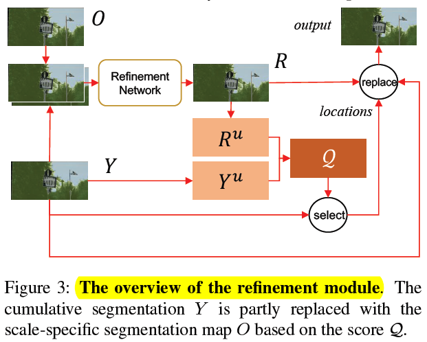
1)refinement module 的输入有两个
- the cumulative result from the previous stages,Y ˉ \bar{Y}Y ˉ
- the result obtained by running the segmentation module at and only at the current scale,O ˉ \bar{O}O ˉ
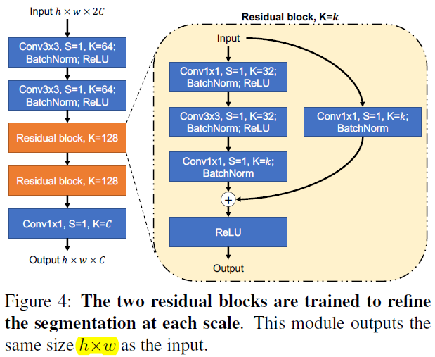
2)refinement network 的结构如下
O+Y=R
3)历史 scale 结果和当前 scale 结果集合
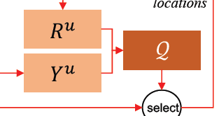
Let Y u Y_u Y u and R u R_u R u denote the prediction uncertainty maps for Y Y Y and R R R respectively.
4)uncertainty maps 的定义为
for each pixel of Y , the prediction confidence at this location is defined as the absolute difference between the highest probability value and the second-highest value (among the C probability values for C classes).
5)使用两个 prediction uncertainty maps来选择 Y Y Y (累积分割图) 的 k k k 个位置进行细化。

- k k k 表示的是Y Y Y 预测的不准确的地方,而R R R预测的比较准确的地方
- ⨀ \bigodot ⨀ 是 element-wise multiplication
- F F F表示中值滤波,用来平滑the score map
- 1 − R 1-R 1 −R 相当于注意力机制,用来对Y Y Y 进行加权
5) Y u Y_u Y u and R u R_u R u 的组合方式为
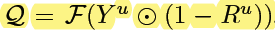
其中 F denotes median blurring to smooth the score map(中值滤波)
⨀ \bigodot ⨀ 是 element-wise multiplication
相当于把 R 的不确定的地方着重更新一下,具体理解方式如下
R R R map 某个 location 分类的越好,softmax 拉的越开,那么 prediction confidence 越大,1-R 越小,就表示不用去 refine 该区域
R R R map 某个 location 分类的越差,softmax 拉不开,那么 prediction confidence 越小,1-R 越大,就表示要着重去 refine 该区域
ps:后续的 select 和 replace 好像分析不出来太多细节,需要再结合代码看看
4.3 MagNetFast
在 MagNet 的基础上
- 减少 scale 数量
- 减少每个 scale 上去 refine 的 patch 数量(only selects the patches with the highest prediction uncertainty Y u Y^u Y u for refinement)
5 Experiments
训练的时候各个 scale 上 randomly extract image patches
测试的时候,extract non-overlapping patches for processing
5.1 Datasets
; 5.2 Experiments on the Cityscapes dataset
1)Benefits of multiple scale levels
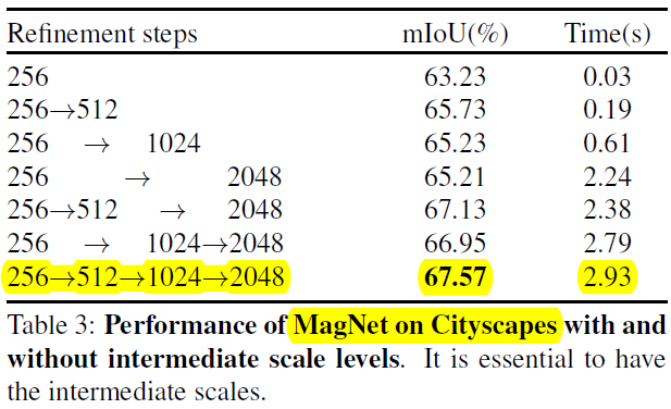
scale 设置为 4 效果最好
这里注意了,patch size 越小,refine 的精度越高
patch size 依次为(hxw)
1024×2048->512×1024->256×512->128×256
网络大小也即 patch resize 的大小为 128×256
相当于 refine 的精度依次为
原图x(128/1024) ->原图x(128/512)->原图x(128/256)->原图x(128/128)
也即
256->512->1024->2048
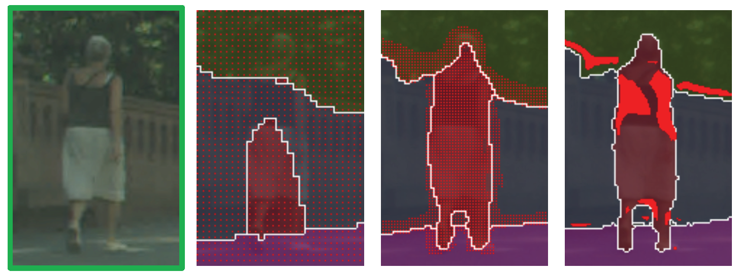
下面感受下效果
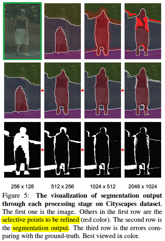
第二行应该是 refine 之后的结果
第一行放大看看,第二张图都是红点
2)Comparing segmentation approaches
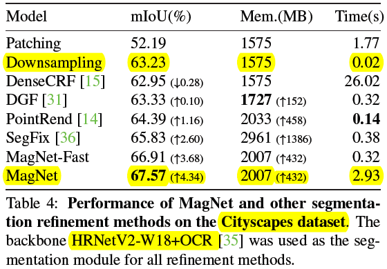
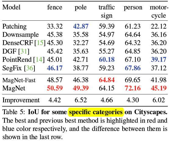
这些类比杆比较多(更细腻),分割的比之前好
3)Ablation study: point selection
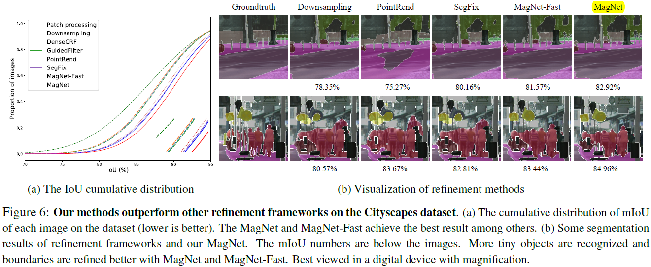
图 (a) 可以看出,MagNet 的 IoU 比其他方法要更大
4)Ablation study: point selection
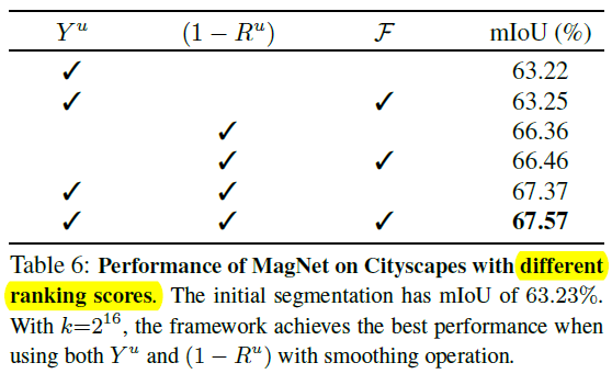
这里探索了一些 Y u Y^u Y u 和 R u R^u R u 的组合方式,2 16 = 65536 2^{16} = 65536 2 1 6 =6 5 5 3 6
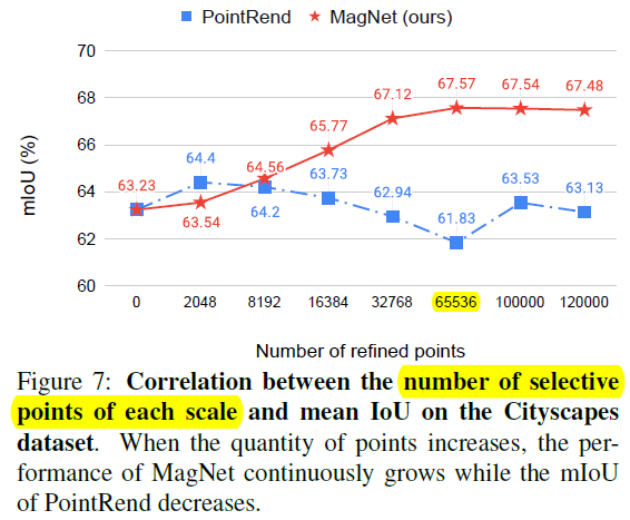
这里探索了一下每个 scale 需要 refine 的 point 数量
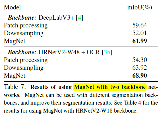
5)Ablation study: segmentation backbones
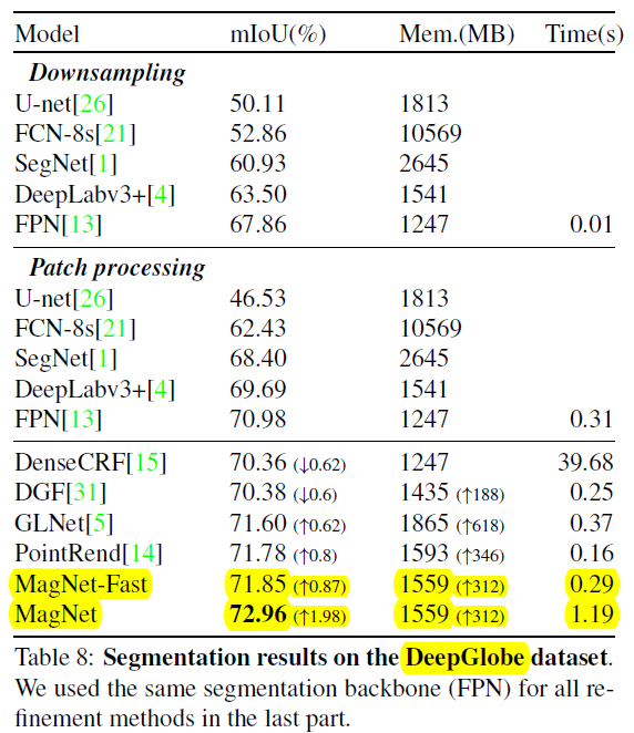
5.3 DeepGlobe
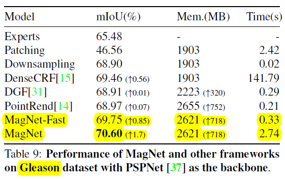
; 5.4 Gleason
6 Conclusion(own)
accumulated 思路不错
stage 过多速度应该会慢很多
细粒度和分辨率
Original: https://blog.csdn.net/bryant_meng/article/details/122185831
Author: bryant_meng
Title: 【MagNet】《Progressive Semantic Segmentation》
原创文章受到原创版权保护。转载请注明出处:https://www.johngo689.com/682621/
转载文章受原作者版权保护。转载请注明原作者出处!