

目录
- 为什么学习pandas
- pandas常用数据类型
- pandas之Series
* - Series的创建
– - Series的切片和索引
- Series的索引和值
- panda读取外部数据
- pandas之DataFrame
* - 创建DataFrame
– - DataFrame的描述信息
- DataFrame排序的方法
- DataFrame的下标索引(loc)和位置索引(iloc)
- pandas的布尔索引
- pandas字符串方法
- pandas缺失数据的处理
- pandas常用统计方法
- panda字符串离散化的案例
- pandas数据的合并和分组类聚
* - 数据的合并 join
- 数据的合并 merge
- 数据的分组聚合 groupby
- pandas索引和复合索引
- 练习
- pandas时间序列
* - 生成一段时间范围 pd.date_range(start,end,periods, freq)
- 将时间戳作为索引
- 将字符串转化为时间戳 pd.to_datetime()
- pandas重采样 t.resample()
- 时间段PeriodIndex
为什么学习pandas
numpy能够帮我们处理处理 数值型数据,但是这还不够;
很多时候,我们的 数据除了数值之外,还有字符串,还有时间序列等
比如:我们通过爬虫获取到了存储在数据库中的数据
比如:之前youtube的例子中除了数值之外还有国家的信息,视频的分类(tag)信息,标题信息等.
所以,numpy能够帮助我们处理数值,但是 pandas除了处理数值之外(基于numpy),还能够帮助我们处理其他类型的数据。
pandas is an open source, BSD-licensed library providing high-performance, easy-to-use data structures and data analysis tools for the Python programming language.
pandas常用数据类型
- Series 一维,带标签数组
- DataFrame 二维,Series容器
pandas之Series
Series的创建
根据列表创建Series
import pandas as pd
t = pd.Series([1,20,13,24,5])
print(t)
print(type(t))

输出:
0     1
1    20
2    13
3    24
4     5
dtype: int64
<class 'pandas.core.series.Series'>
指定Series的索引
import string
import pandas as pd
t = pd.Series(range(10), index=list(string.ascii_uppercase[:10]))
print(t)
print(type(t))

输出:
A    0
B    1
C    2
D    3
E    4
F    5
G    6
H    7
I    8
J    9
dtype: int64
<class 'pandas.core.series.Series'>
根据字典创建Series
import pandas as pd
temp_dict = dict(name = 'sherry', age = 24, sex = 'female')
t = pd.Series(temp_dict)
print(t)
print(type(t))

输出:
name    sherry
age         24
sex     female
dtype: object
<class 'pandas.core.series.Series'>
import string
import pandas as pd

t = pd.Series({string.ascii_uppercase[i]:i for i in range(10)})
print(t)
print(type(t))

t2 = pd.Series(t, index = list(string.ascii_uppercase[5:15]))
print(t2)

输出:
A    0
B    1
C    2
D    3
E    4
F    5
G    6
H    7
I    8
J    9
dtype: int64
<class 'pandas.core.series.Series'>
F    5.0
G    6.0
H    7.0
I    8.0
J    9.0
K    NaN
L    NaN
M    NaN
N    NaN
O    NaN
dtype: float64
修改Series的dtype类型
t.astype(dtype)
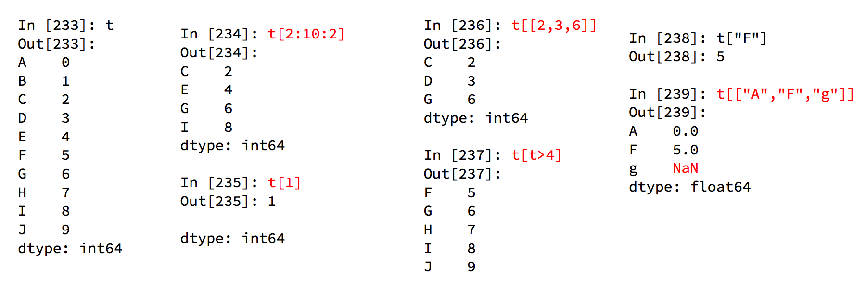
Series的切片和索引
和numpy操作一样。

import pandas as pd
temp_dict = dict(name = 'sherry', age = 24, sex = 'female')
t = pd.Series(temp_dict)
print(t)
print(type(t))

print('*'*20)
print('通过index索引')
print(t['name'])
print(t['age'])

print('*'*20)
print('通过位置索引')
print(t[0])
print(t[1])

print('*'*20)
print('根据多个index索引多个值')
print(t[['name', 'age']])

print('*'*20)
print('根据多个位置索引多个值')
print(t[[0,2]])

print('*'*10)
print('切片操作')
print(t[:1])

输出:
name    sherry
age         24
sex     female
dtype: object
<class 'pandas.core.series.Series'>
********************
通过index索引
sherry
24
********************
通过位置索引
sherry
24
********************
根据多个index索引多个值
name    sherry
age         24
dtype: object
********************
根据多个位置索引多个值
name    sherry
sex     female
dtype: object
**********
切片操作
name    sherry
dtype: object
Series的索引和值
属性:
t.index
t.values
import pandas as pd
temp_dict = dict(name = 'sherry', age = 24, sex = 'female')
t = pd.Series(temp_dict)

print('t.index\t\t',t.index)
print('type(t.index)\t',type(t.index))
print('list(t.index)\t',list(t.index))
print('t.values\t',t.values)
print('type(t.values)\t',type(t.values))

输出:
t.index          Index(['name', 'age', 'sex'], dtype='object')
type(t.index)    <class 'pandas.core.indexes.base.Index'>
list(t.index)    ['name', 'age', 'sex']
t.values         ['sherry' 24 'female']
type(t.values)   <class 'numpy.ndarray'>
ndarray(numpy数组很多方法,都可以运用于Series类型,比如argmax, clip等),但是Series的where方法和numpy不同。
panda读取外部数据
现在假设我们有一个组关于狗的名字的统计数据,那么为了观察这组数据的情况,我们应该怎么做呢?

import pandas as pd
data = pd.read_csv('./dogNames2.csv')
print(data)
print(type(data))

输出:
      Row_Labels  Count_AnimalName
0              1                 1
1              2                 2
2          40804                 1
3          90201                 1
4          90203                 1
...          ...               ...

16215      37916                 1
16216      38282                 1
16217      38583                 1
16218      38948                 1
16219      39743                 1

[16220 rows x 2 columns]
<class 'pandas.core.frame.DataFrame'>
读取数据库:
pd.read_sql(sql_sentence,connection)
pandas之DataFrame
创建DataFrame
传入数组,创建DataFrame
import pandas as pd
import numpy as np
t = pd.DataFrame(np.arange(12).reshape(3,4))
print(t)

输出:
   0  1   2   3
0  0  1   2   3
1  4  5   6   7
2  8  9  10  11
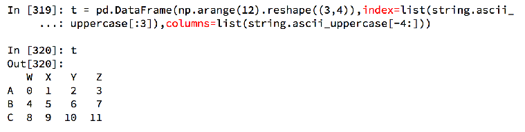
指定DataFrame的行索引index和列索引columns
DataFrame对象既有行索引,又有列索引:
行索引,代表不同行,横向索引,叫index,0轴,axis=0
列索引,代表不同列,纵向索引,叫columns,1轴,axis=1
import pandas as pd
import numpy as np
t = pd.DataFrame(np.arange(12).reshape(3,4), index = ['a','b','c'], columns=['W','X','Y','Z'])
print(t)

输出:
   W  X   Y   Z
a  0  1   2   3
b  4  5   6   7
c  8  9  10  11
根据字典创建DataFrame
字典键值对应列表,或者列表元素是字典。另外,如果传入字典元素值为空,则DataFrame中对应值为nan。
import pandas as pd

d1 = dict(name = ['sherry','lily','logan'], age = [24,25,30])
t = pd.DataFrame(d1)
print(t)

d2 = [dict(name='xiaowang', age = 24), dict(name = 'xiaohong', age = 25), dict(name='xiaoming')]
t2 = pd.DataFrame(d2)
print(t2)

输出:
     name  age
0  sherry   24
1    lily   25
2   logan   30
       name   age
0  xiaowang  24.0
1  xiaohong  25.0
2  xiaoming   NaN
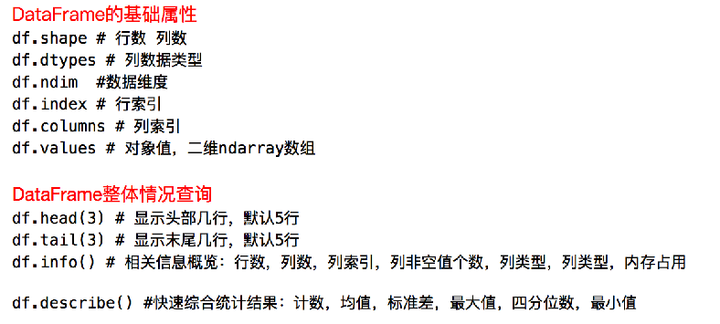
DataFrame的描述信息
import pandas as pd
d1 = dict(name = ['sherry','lily','logan'], age = [24,25,30])
t = pd.DataFrame(d1)
print(t)
print('*'*30)
print('index:\t\t',t.index)
print('columns:\t',t.columns)
print('values:\n',t.values)
print('shape:\t\t',t.shape)
print('dtypes:\n',t.dtypes)
print('ndim:\t\t',t.ndim)
print('*'*30)
print(t.head(1))
print('*'*30)
print(t.tail(1))
print('*'*30)
print('info:')
print(t.info())
print('*'*30)
print('describle:')
print(t.describe())

输出:
     name  age
0  sherry   24
1    lily   25
2   logan   30
******************************
index:           RangeIndex(start=0, stop=3, step=1)
columns:         Index(['name', 'age'], dtype='object')
values:
 [['sherry' 24]
 ['lily' 25]
 ['logan' 30]]
shape:           (3, 2)
dtypes:
 name    object
age      int64
dtype: object
ndim:            2
******************************
     name  age
0  sherry   24
******************************
    name  age
2  logan   30
******************************
info:
<class 'pandas.core.frame.DataFrame'>
RangeIndex: 3 entries, 0 to 2
Data columns (total 2 columns):

 0   Rank                1000 non-null   int64
 1   Title               1000 non-null   object
 2   Genre               1000 non-null   object
 3   Description         1000 non-null   object
 4   Director            1000 non-null   object
 5   Actors              1000 non-null   object
 6   Year                1000 non-null   int64
 7   Runtime (Minutes)   1000 non-null   int64
 8   Rating              1000 non-null   float64
 9   Votes               1000 non-null   int64
 10  Revenue (Millions)  872 non-null    float64
 11  Metascore           936 non-null    float64
dtypes: float64(3), int64(4), object(5)
memory usage: 93.9+ KB
None
6.723200000000003
644
644
2394
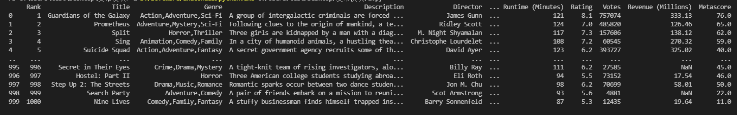
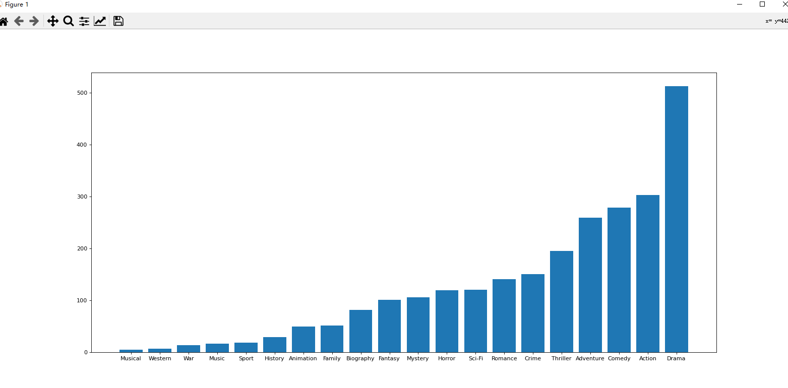
panda字符串离散化的案例
对于一组电影数据,如果我们希望统计电影分类(genre)的情况,应该如何处理数据?
思路:重新构造一个全为0的数组,列名为分类,如果某一条数据中分类出现过,就让0变为1;
import pandas as pd
import numpy as np
from matplotlib import pyplot as plt

df = pd.read_csv('IMDB-Movie-Data.csv')
genre_data = df['Genre']
temp_list = genre_data.str.split(',').tolist()
genre_list = list(set([i for j in temp_list for i in j]))
num_datas = df.count()

zeros_df = pd.DataFrame(np.zeros((df.shape[0], len(genre_list))), columns=genre_list)

for i in range(df.shape[0]):
    zeros_df.loc[i,temp_list[i]] = 1

genre_count = zeros_df.sum(axis=0)
print(genre_count)

genre_count = genre_count.sort_values()

plt.figure(figsize=(20,9), dpi =80)
plt.bar(range(len(genre_count.index)),genre_count.values)
plt.xticks(range(len(genre_count.index)),genre_count.index)
plt.show()
结果:
pandas数据的合并和分组类聚
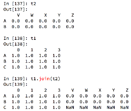
数据的合并 join
join:默认情况下他是把 行索引相同的数据合并到一起;要求列索引不重复,这样就只copy行数据到相同的行索引数据上。等于 水平拼接。
import pandas as pd
import numpy as np

df1 = pd.DataFrame(np.arange(12,20).reshape(2,4), index = list('AB'),columns=list('abcd'))
df2 = pd.DataFrame(np.arange(9).reshape(3,3), index = list('BAC'),columns=list('xyz'))
print(df1)
print(df2)
print(df1.join(df2))

输出:
    a   b   c   d
A  12  13  14  15
B  16  17  18  19
   x  y  z
B  0  1  2
A  3  4  5
C  6  7  8
    a   b   c   d  x  y  z
A  12  13  14  15  3  4  5
B  16  17  18  19  0  1  2
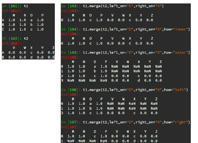
数据的合并 merge
merge: 按照指定的列把数据按照一定的方式合并到一起 的,等于是指定列索引合并行数据。
默认的合并方式inner,交集;
merge outer并集,NaN补全;
merge left,左边为准,NaN补全;
merge right,右边为准,NaN补全;
merge合并操作和数据库连接操作。
import pandas as pd
import numpy as np
from matplotlib import pyplot as plt

df1 = pd.DataFrame(np.arange(12,20).reshape(2,4), index = list('AB'),columns=list('abcd'))
df2 = pd.DataFrame(np.arange(9).reshape(3,3), columns=list('fax'))
df1.loc[:,'a'] = 1
print('*'*40)
print(df1)
print(df2)

print('*'*40)
t1 = df1.merge(df2)
print(t1)

t2 = df1.merge(df2, on = 'a')
print(t2)

df1.loc['B','a'] = 100
t2 = df1.merge(df2, on = 'a')
print(t2)

print('*'*40)
t3 = df1.merge(df2, on='a', how = 'outer')
print(t3)

print('*'*40)
t4 = df1.merge(df2, on='a', how = 'left')
print(t4)
t5 = df1.merge(df2, on='a', how = 'right')
print(t5)

输出:
****************************************
   a   b   c   d
A  1  13  14  15
B  1  17  18  19
   f  a  x
0  0  1  2
1  3  4  5
2  6  7  8
****************************************
   a   b   c   d  f  x
0  1  13  14  15  0  2
1  1  17  18  19  0  2
   a   b   c   d  f  x
0  1  13  14  15  0  2
1  1  17  18  19  0  2
   a   b   c   d  f  x
0  1  13  14  15  0  2
****************************************
     a     b     c     d    f    x
0    1  13.0  14.0  15.0  0.0  2.0
1  100  17.0  18.0  19.0  NaN  NaN
2    4   NaN   NaN   NaN  3.0  5.0
3    7   NaN   NaN   NaN  6.0  8.0
****************************************
     a   b   c   d    f    x
0    1  13  14  15  0.0  2.0
1  100  17  18  19  NaN  NaN
   a     b     c     d  f  x
0  1  13.0  14.0  15.0  0  2
1  4   NaN   NaN   NaN  3  5
2  7   NaN   NaN   NaN  6  8
数据的分组聚合 groupby
在pandas中类似的分组的操作我们有很简单的方式来完:
grouped = df.groupby(by=”columns_name”)
grouped是一个DataFrameGroupBy对象,是可迭代的
grouped中的 每一个元素是一个元组;
元组里面是( 索引(分组的值),分组之后的DataFrame);
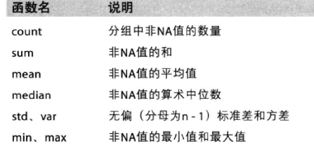
DataFrameGroupBy对象有很多经过优化的方法(聚合):
import pandas as pd
df = pd.read_csv('./starbucks_store_worldwide.csv')

grouped = df.groupby(by='Country')

country_count = grouped['Brand'].count()
print(country_count['US'])
print(country_count['CN'])

china_data = df[df['Country']=='CN']
grouped = china_data.groupby(by='State/Province')['Brand'].count()
print(grouped)

输出:
13608
2734
State/Province
11    236
12     58
13     24
14      8
15      8
21     57
22     13
23     16
31    551
32    354
33    315
...
如果我们需要对国家和省份进行分组统计,应该怎么操作呢?
grouped = df.groupby(by=[“Country”,”State/Province”])
很多时候我们只希望对获取分组之后的某一部分数据,或者说我们只希望对某几列数据进行分组,这个时候我们应该怎么办呢?
获取分组之后的某一部分数据:
df.groupby(by=[“Country”,”State/Province”])[“Country”].count() 返回Series
对某几列数据进行分组: 这里必须是df[“Country”],df[“State/Province”],因为df[“Country”]没有列Country和State/Province。
df[“Country”].groupby(by=[df[“Country”],df[“State/Province”]]).count()返回Series
观察结果,由于只选择了一列数据,所以结果是一个Series类型
如果我想返回一个DataFrame类型呢?
t1 = df[[“Country”]].groupby(by=[df[“Country”],df[“State/Province”]]).count()
t2 = df.groupby(by=[“Country”,”State/Province”])[[“Country”]].count()
t3 = df.groupby(by=[“Country”,”State/Province”]).count().[[“Country”]]
上面三条语句返回的都是DataFrame类型。
pandas索引和复合索引
简单的索引操作:
获取index:df.index
指定index :df.index = [‘x’,’y’]
重新设置index : df.reindex(list(“abcedf”))
指定某一列的值作为index:df.set_index(“Country”,drop=False)
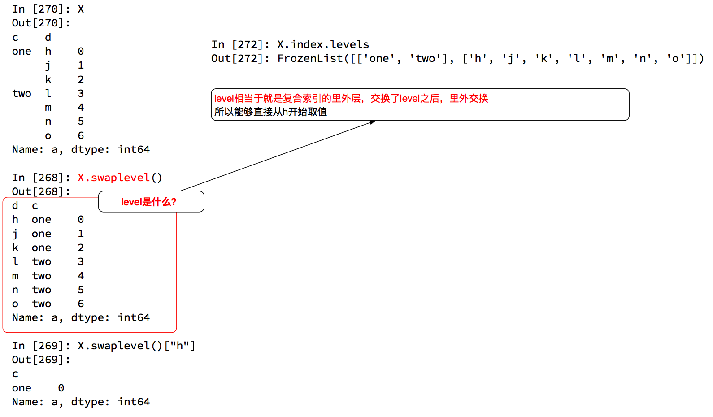
返回index的唯一值:df.set_index(“Country”).index.unique()【Pandas中索引可重复】设置两列的值为索引(复合索引): a.set_index([“c”,”d”])
复合索引中,Series直接通过t[索引1,索引2,…]索引值,DataFrame通过t.loc[索引1].loc[索引2]索引值。
import pandas as pd
import numpy as np

df1 = pd.DataFrame(np.arange(12,20).reshape(2,4), index = list('AB'),columns=list('abcd'))

print('*'*30)
print(df1.index)
df1.index = list('CD')
print(df1)

print('*'*30)
df2 = df1.reindex(['C','DD'])
print(df2)
print(df2.index)

print('*'*30)
df3 = df1.set_index('a')
print(df3)
print(df3.index)
print('*'*30)
df3 = df1.set_index('a',drop = False)
print(df3)

print('*'*30)
print(df3.index.unique())

print('*'*30)
print(len(df3.index))

print('*'*30)
df4 = df1.set_index(['a','b'])
print(df4)
print(df4.index)

print('*'*30)
df5 = df1.set_index(['a','b','c'])
print(df5)
print(df5.index)

输出:
******************************
Index(['A', 'B'], dtype='object')
    a   b   c   d
C  12  13  14  15
D  16  17  18  19
******************************
       a     b     c     d
C   12.0  13.0  14.0  15.0
DD   NaN   NaN   NaN   NaN
Index(['C', 'DD'], dtype='object')
******************************
     b   c   d
a
12  13  14  15
16  17  18  19
Int64Index([12, 16], dtype='int64', name='a')
******************************
     a   b   c   d
a
12  12  13  14  15
16  16  17  18  19
******************************
Int64Index([12, 16], dtype='int64', name='a')
******************************
2
******************************
        c   d
a  b
12 13  14  15
16 17  18  19
MultiIndex([(12, 13),
            (16, 17)],
           names=['a', 'b'])
******************************
           d
a  b  c
12 13 14  15
16 17 18  19
MultiIndex([(12, 13, 14),
            (16, 17, 18)],
           names=['a', 'b', 'c'])
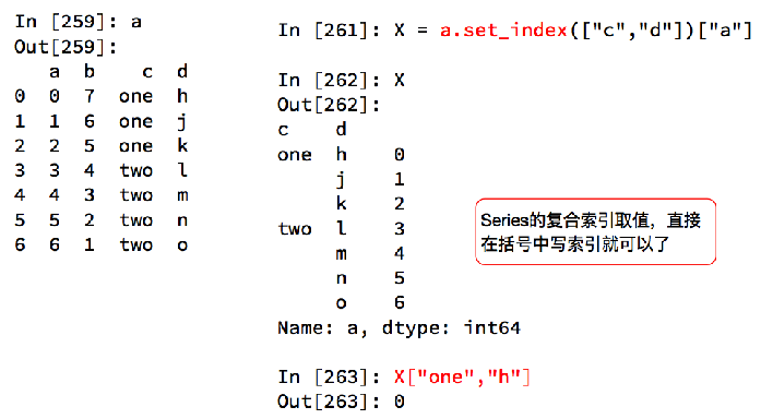
import pandas as pd
import numpy as np

a = pd.DataFrame({'a': range(7),'b': range(7, 0, -1),'c': ['one','one','one','two','two','two', 'two'],'d': list("hjklmno")})
print(a)
b = a.set_index(['c','d'])
print(b)

print('*'*20)

c = b["a"]
print(c)
print(type(c))
print(c['one','k'])

print('*'*20)

print(b.loc['one'])
print(b.loc['one'].loc['k'])

输出:
   a  b    c  d
0  0  7  one  h
1  1  6  one  j
2  2  5  one  k
3  3  4  two  l
4  4  3  two  m
5  5  2  two  n
6  6  1  two  o
       a  b
c   d
one h  0  7
    j  1  6
    k  2  5
two l  3  4
    m  4  3
    n  5  2
    o  6  1
********************
c    d
one  h    0
     j    1
     k    2
two  l    3
     m    4
     n    5
     o    6
Name: a, dtype: int64
<class 'pandas.core.series.Series'>
2
********************
   a  b
d
h  0  7
j  1  6
k  2  5
a    2
b    5
Name: k, dtype: int64
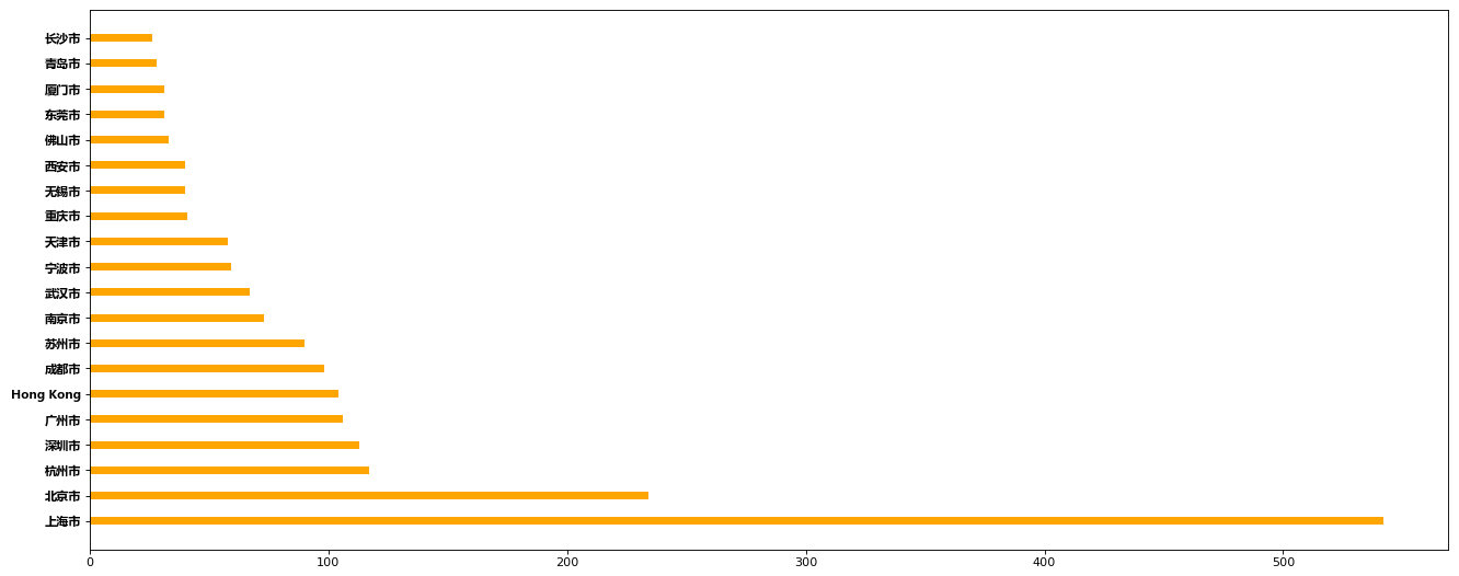
练习
使用matplotlib呈现出每个中国每个城市的店铺数量
from turtle import color
import pandas as pd
from matplotlib import pyplot as plt
from matplotlib import font_manager
my_font = font_manager.FontProperties(fname='C:/WINDOWS/Fonts/msyhbd.ttc')
df = pd.read_csv('./starbucks_store_worldwide.csv')

data = df[df['Country']=='CN'].groupby('City').count().sort_values(by='Brand', ascending=False)[:20]
plt.figure(figsize=(20,8), dpi = 80)
plt.barh(data.index, data['Brand'], height=0.3, color='orange')
plt.yticks(fontproperties=my_font)
plt.show()
结果:
pandas时间序列
不管在什么行业,时间序列都是一种非常重要的数据形式,很多统计数据以及数据的规律也都和时间序列有着非常重要的联系;而且在pandas中处理时间序列是非常简单的。
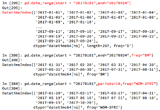
生成一段时间范围 pd.date_range(start,end,periods, freq)
pd.date_range(start=None, end=None, periods=None, freq=’D’)
产生一些列时间戳。类型为DatetimeIndex。
start和end以及freq配合能够生成start和end范围内以频率freq的一组时间索引
start和periods以及freq配合能够生成从start开始的频率为freq的periods个时间索引
频率的缩写:
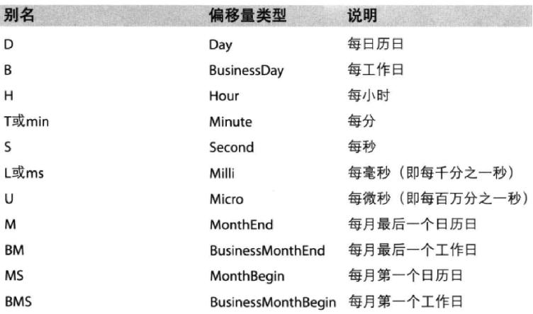
; 将时间戳作为索引
index=pd.date_range(“20170101”,periods=10)
df = pd.DataFrame(np.random.rand(10),index=index)
将字符串转化为时间戳 pd.to_datetime()
可以使用pandas提供的方法把时间字符串转化为时间序列:
df[“timeStamp”] = pd.to_datetime(df[“timeStamp”],format=””)
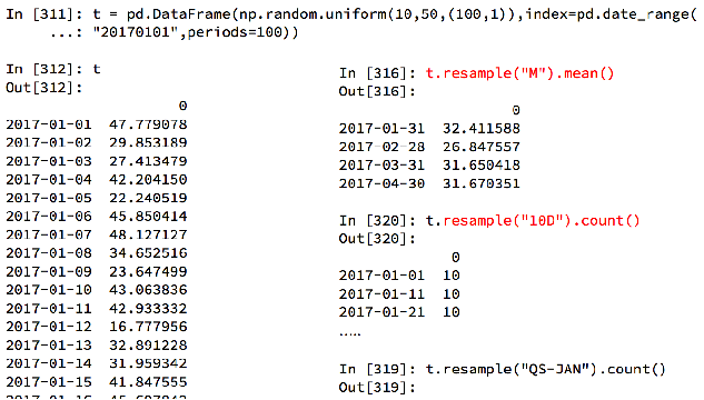
pandas重采样 t.resample()
重采样:指的是将时间序列从一个频率转化为另一个频率进行处理的过程,将高频率数据转化为低频率数据为 降采样,低频率转化为高频率为 升采样。
pandas提供了一个resample的方法来帮助我们实现频率转化。
t为data_time类型作为索引的DataFrame:
t.resample(‘M’).mean() 按月统计平均值
t.resample(’10D’).count() 每10天统计一次数量。
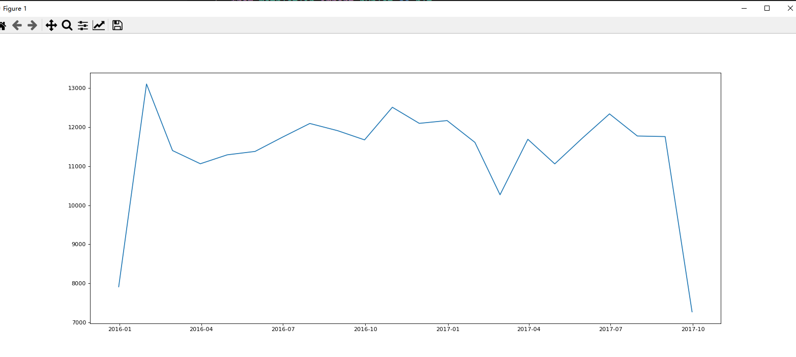
统计出911数据中不同月份电话次数的变化情况:
import pandas as pd
import numpy as np
from matplotlib import pyplot as plt
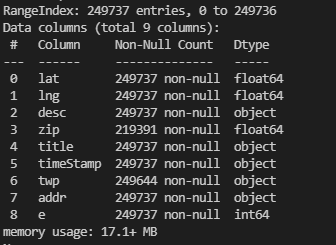
df = pd.read_csv('911.csv')
print(df.info())
df['timeStamp'] = pd.to_datetime(df['timeStamp'])
df.set_index('timeStamp', inplace=True)
count_by_month = df.resample('M').count()['title']
plt.figure(figsize=(20,8), dpi=80)
plt.plot(count_by_month.index, count_by_month)
plt.show()
print(count_by_month.index)
结果:
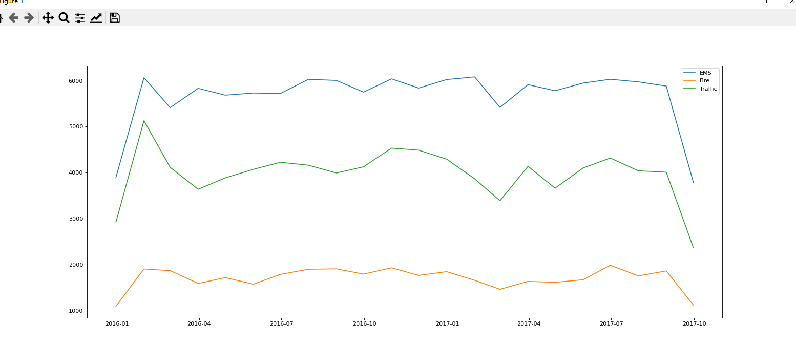
统计出911数据中不同月份不同类型的电话的次数的变化情况
import pandas as pd
import numpy as np
from matplotlib import pyplot as plt

def plot_img(df, label):
    count_by_month = df.resample('M').count()['title']
    plt.plot(count_by_month.index, count_by_month, label = label)

df = pd.read_csv('911.csv')
print(df.info())

temp_list = df['title'].str.split(': ').to_list()
cate_list = [i[0] for i in temp_list]
df["cate"] = pd.DataFrame(np.array(cate_list).reshape((df.shape[0],1)))

df["cate"] = cate_list

df['timeStamp'] = pd.to_datetime(df['timeStamp'])
df.set_index('timeStamp', inplace=True)

plt.figure(figsize=(20,8), dpi=80)

grouped = df.groupby(by='cate')
for group_name, group_data in grouped:

    plot_img(group_data, group_name)

plt.legend(loc='best')
plt.show()
结果:
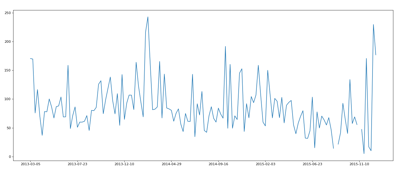
时间段PeriodIndex
之前所学习的DatetimeIndex可以理解为时间戳;
那么PeriodIndex可以理解为时间段;
periods = pd.PeriodIndex(year=data[“year”],month=data[“month”],day=data[“day”],hour=data[“hour”],freq=”H”)

import pandas as pd
import numpy as np
from matplotlib import pyplot as plt

df = pd.read_csv('pm2.5/BeijingPM20100101_20151231.csv')

period = pd.PeriodIndex(year = df['year'], month = df['month'], day = df['day'], hour = df['hour'], freq = 'H')

df['period'] = period
df.set_index('period', inplace=True)
print(df)

df.dropna(axis=0, inplace=True)
df =df.resample('7D').mean()

print(df.head())
data = df['PM_US Post']

x = data.index
x_labels = [i.strftime("%Y-%m-%d") for i in x]
y = data.values

plt.figure(figsize=(20,8), dpi = 80)
plt.plot(range(len(x)), y)
plt.xticks(range(0,len(x),20), x_labels[::20])
plt.show()
结果:
Original: https://blog.csdn.net/sherryhwang/article/details/123133955
Author: sherryhwang
Title: 数据分析(三)- pandas基础
原创文章受到原创版权保护。转载请注明出处:https://www.johngo689.com/674930/
转载文章受原作者版权保护。转载请注明原作者出处!