

【神经网络与深度学习-TensorFlow实践】-中国大学MOOC课程(十一)(分类问题))
- 11 分类问题
* - 11.1 逻辑回归
– - 11.2 实例:实现一元逻辑回归
–- 11.2.1 sigmoid()函数-代码实现
- 11.2.2 交叉熵损失函数-代码实现
- 11.2.3 准确率-代码实现
+ - 11.2.3.1 判断阈值是0.5-tf.round()函数
- 11.2.3.2 判断阈值不是0.5–where(condition,a,b)函数
- 11.2.4 一元逻辑回归-房屋销售记录实例
+ - 11.2.4.1 加载数据
- 11.2.4.2 数据处理
- 11.2.4.3 设置超参数
- 11.2.4.4 设置模型变量初始值
- 11.2.4.5 训练模型
- 11.2.4.6 增加sigmoid曲线可视化输出
- 11.2.4.7 验证模型
- 11.2.4.8 预测值的sigmoid曲线和散点图
- 11.3 线性分类器(Linear Classifier)
– - 11.4 实例:实现多元逻辑回归
– - 11.5 多分类问题
– - 11.6 实例:多分类问题
– - 11.7 参考文献
11 分类问题
11.1 逻辑回归
11.1.1 广义线性回归
-
课程回顾
-
线性回归:将自变量和因变量之间的关系,用线性模型来表示;根据已知的样本数据,对未来的、或者未知的数据进行估计
-
对数线性回归(log-linear regression)
lny = wx+b 即:y=ewx+b
Y= wx+b
g(y) = wx+b 也即:y=h(wx+b)
y = g-1(wx+b) -
*广义线性模型(generalized linear model)
-
g(·):联系函数(link function),任何单调可微函数
-
高维模型 Y = g-1(WTX)
W = (w0,w1,…,wm)T
X = (x0,x1,…,xm)T
x0=1
11.1.2 逻辑回归
11.1.2.1 分类问题
- 分类问题:垃圾邮件识别,图片分类,疾病判断
- 分类器:能偶自动对输入的数据进行分类
输入: 特征;输出: *离散值
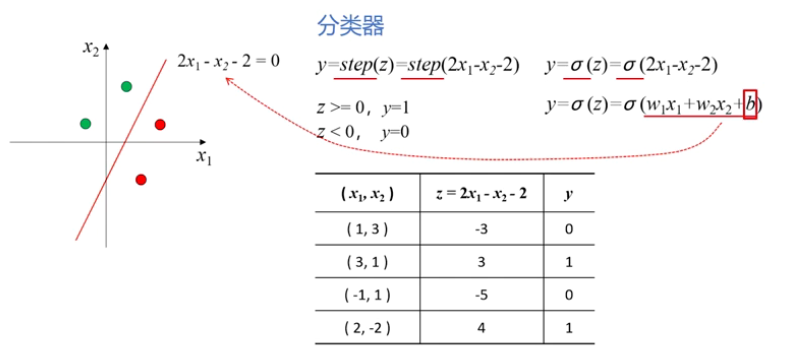
11.1.2.2 实现分类器
- 准备训练样本
- 训练分类器
- 对新样本分类
- 单位阶跃函数(unit-step function)
不光滑
不连续 - 二分类问题 1/0–正例和反例
- 对数几率函数(logistic function):y=1/(1+e-z)
单调上升,连续,光滑
任意阶可导 - 对数几率回归/逻辑回归(logistic regression):y=1/(1+e-(wx+b))
- Sigmoid函数:形状s的函数,能够将取值范围无穷大的函数转化为一个0到1范围的值;
y=g-1(z)=σ(z)=σ(wx+b)=1/(1+e-z)=1/(1+e-(wx+b)) - 多元模型
y = 1/(1+e-(W^TX))
W = (w0,w1,…,wm)T
X = (x0,x1,…,xm)T
x0=1
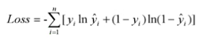
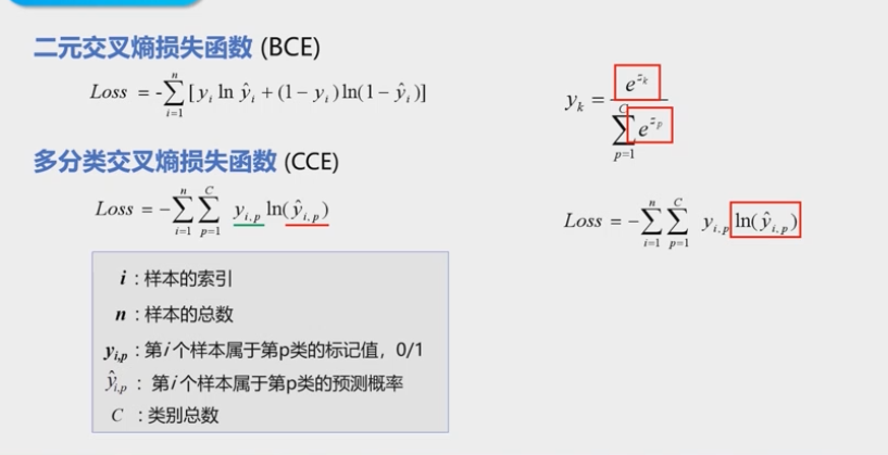
11.1.3 交叉熵损失函数
-
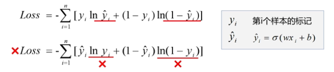
交叉熵损失函数
-
每一项误差都是非负的
- 函数值和误差的变化趋势一致
- 凸函数
-
对模型参数求偏导数,无σ'()项

-
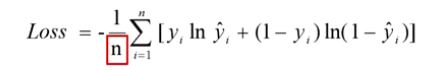
平均交叉熵损失函数
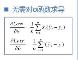
- 偏导数的值只受到标签值和预测值偏差的影响
- 交叉熵损失函数是凸函数,因此使用梯度下降法得到的极小值就是全局最小值
; 11.1.4 准确率(accuracy)
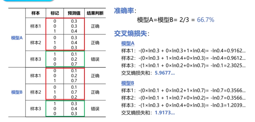
- 可以使用准确率来评价一个分类器性能
- 准确率=正确分类的样本数/总样本数
- 仅仅通过准确率是无法细分出模型分类器的优劣的
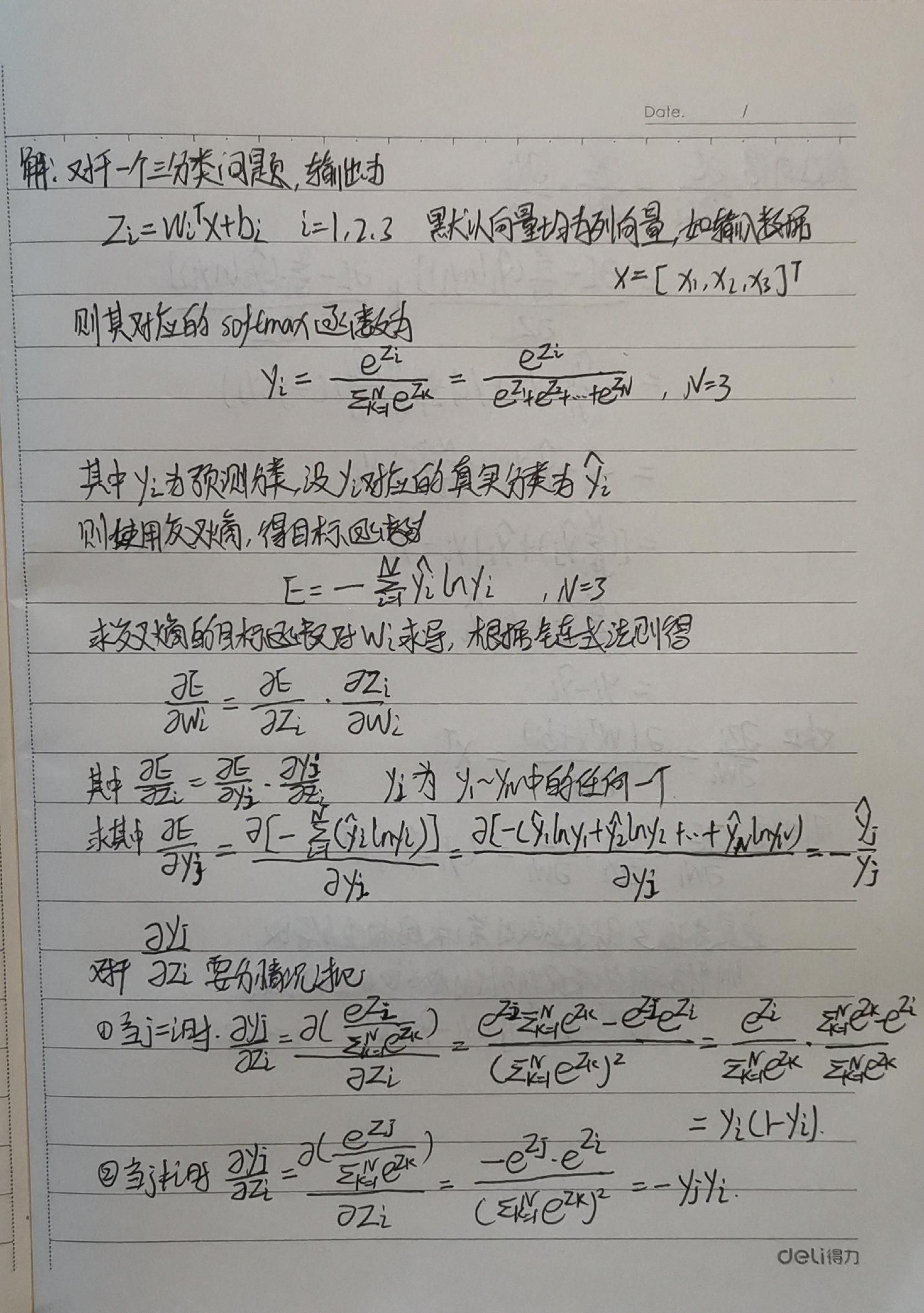
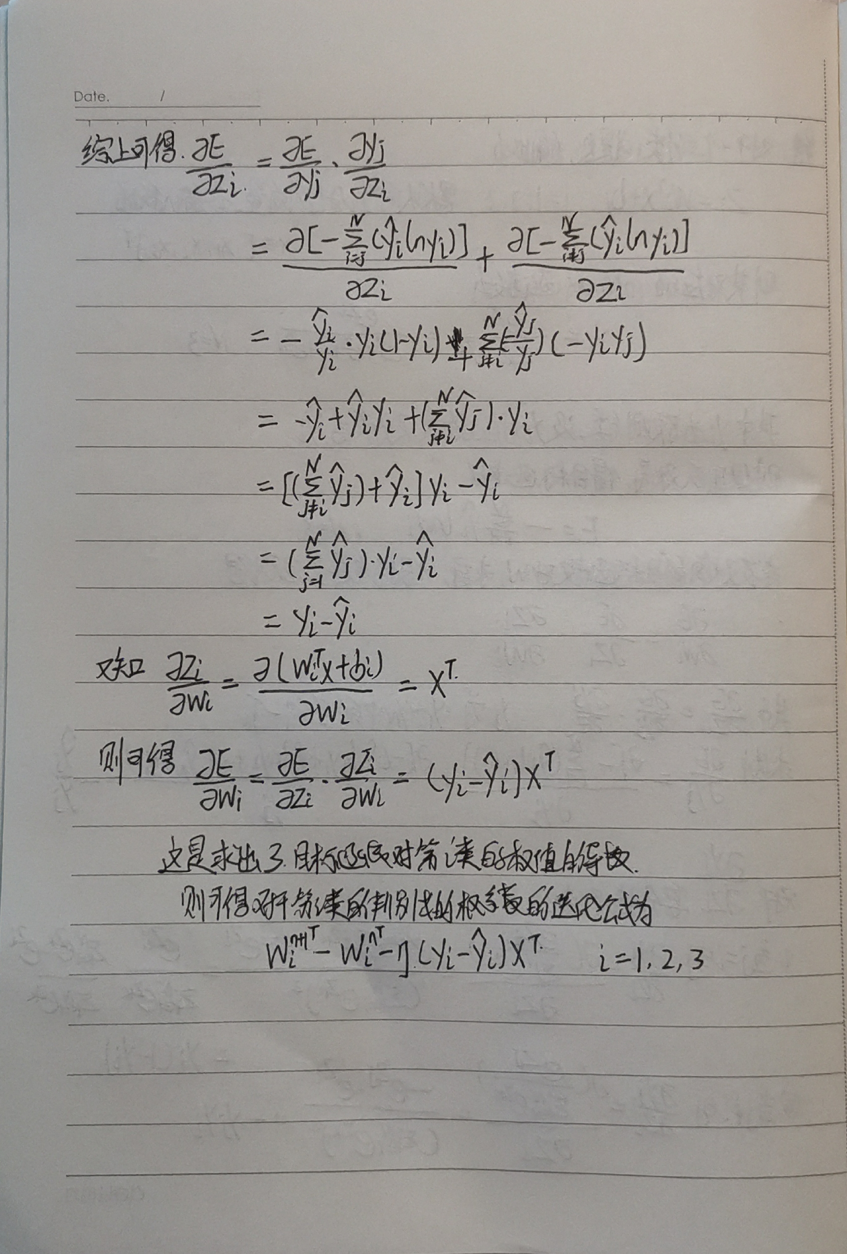
11.1.5 手推三分类问题-交叉熵损失函数,权值更新公式
; 11.2 实例:实现一元逻辑回归
11.2.1 sigmoid()函数-代码实现
y = 1 / ( 1 + e-(wx+b))
>>> import tensorflow as tf
>>> import numpy as np
>>> x = np.array([1.,2.,3.,4.])
>>> w = tf.Variable(1.)
>>> b = tf.Variable(1.)
>>> y = 1/(1+tf.exp(-(w*x+b)))
>>> y
<tf.Tensor: id=46, shape=(4,), dtype=float32, numpy=array([0.880797  , 0.95257413, 0.98201376, 0.9933072 ], dtype=float32)>
- *注意tf.exp()函数的参数要求是浮点数,否则会报错
11.2.2 交叉熵损失函数-代码实现
>>> import tensorflow as tf
>>> import numpy as np

>>> y = np.array([0,0,1,1])
>>> pred=np.array([0.1,0.2,0.8,0.49])

>>>
>>> -tf.reduce_sum(y*tf.math.log(pred)+(1-y)*tf.math.log(1-pred))
<tf.Tensor: id=58, shape=(), dtype=float64, numpy=1.2649975061637104>

>>>
>>> -tf.reduce_mean(y*tf.math.log(pred)+(1-y)*tf.math.log(1-pred))
<tf.Tensor: id=70, shape=(), dtype=float64, numpy=0.3162493765409276>
11.2.3 准确率-代码实现
11.2.3.1 判断阈值是0.5-tf.round()函数
- 准确率=正确分类的样本数/总样本数
>>> import tensorflow as tf
>>> import numpy as np

>>> y = np.array([0,0,1,1])
>>> pred=np.array([0.1,0.2,0.8,0.49])

>>>
>>> tf.round(pred)
<tf.Tensor: id=83, shape=(4,), dtype=float64, numpy=array([0., 0.,
1., 0.])>

>>>
和y形状相同的一维张量
>>> tf.equal(tf.round(pred),y)
<tf.Tensor: id=87, shape=(4,), dtype=bool, numpy=array([ True,  True,  True, False])>

>>>
>>> tf.cast(tf.equal(tf.round(pred),y),tf.int8)
<tf.Tensor: id=92, shape=(4,), dtype=int8, numpy=array([1, 1, 1, 0], dtype=int8)>

>>>
>>> tf.reduce_mean(tf.cast(tf.equal(tf.round(pred),y),tf.int8))
<tf.Tensor: id=99, shape=(), dtype=int8, numpy=0>

>>>
>>> tf.round(0.5)
<tf.Tensor: id=101, shape=(), dtype=float32, numpy=0.0>
11.2.3.2 判断阈值不是0.5–where(condition,a,b)函数
where(condition,a,b)
- 根据条件condition返回a或者b的值
- 如果condition中的某个元素为真,对应位置返回a,否则返回b
>>> import tensorflow as tf
>>> import numpy as np

>>> y = np.array([0,0,1,1])
>>> pred=np.array([0.1,0.2,0.8,0.49])

>>> tf.where(pred<0.5,0,1)
<tf.Tensor: id=105, shape=(4,), dtype=int32, numpy=array([0, 0, 1,
0])>

>>> pred<0.5
array([ True,  True, False,  True])

>>> tf.where(pred<0.4,0,1)
- 参数a和b还可以是数组或者张量,这时,a和b必须有相同的形状,并且他们的第一维必须和condition形状一致
>>> import tensorflow as tf
>>> import numpy as np

>>> pred=np.array([0.1,0.2,0.8,0.49])

>>> a = np.array([1,2,3,4])
>>> b = np.array([10,20,30,40])

>>>
>>> tf.where(pred<0.5,a,b)
<tf.Tensor: id=117, shape=(4,), dtype=int32, numpy=array([ 1,  2, 30,  4])>
>>>
,而第3个元素大于0.5,取b中的元素
- 参数a和b也可以省略,这时的返回值数组pred中大于等于0.5的元素的索引,返回值以一个二维张量的形式给出
>>> tf.where(pred>=0.5)
<tf.Tensor: id=119, shape=(1, 1), dtype=int64, numpy=array([[2]], dtype=int64)>
*下面使用where计算准确率
>>> import tensorflow as tf
>>> import numpy as np
>>> y = np.array([0,0,1,1])
>>> pred=np.array([0.1,0.2,0.8,0.49])

>>> tf.reduce_mean(tf.cast(tf.equal(tf.where(pred<0.5,0,1),y),tf.float32))
<tf.Tensor: id=136, shape=(), dtype=float32, numpy=0.75>
11.2.4 一元逻辑回归-房屋销售记录实例
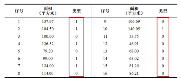
- 0:普通住宅;1:高档住宅
; 11.2.4.1 加载数据
import tensorflow as tf
import numpy as np
import matplotlib.pyplot as plt
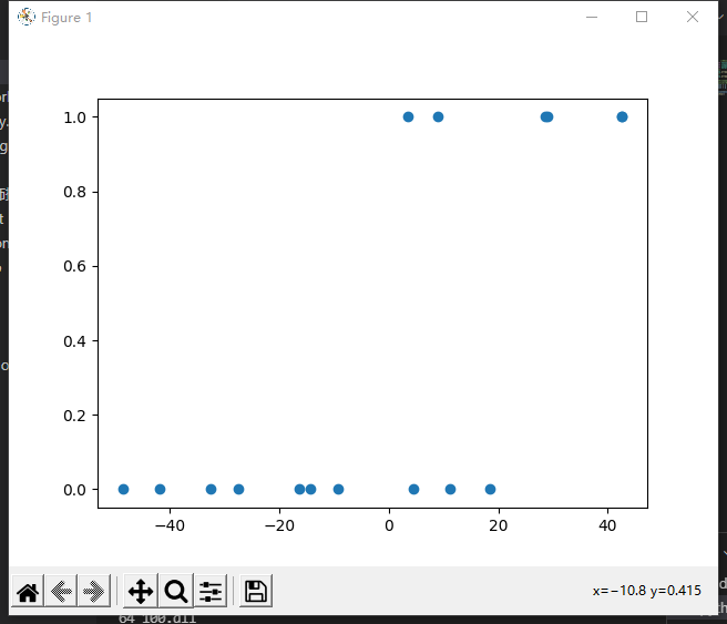
x = np.array([137.97,104.50,100.00,124.32,79.20,99.00,124.00,114.00,106.69,138.05,53.75,46.91,68.00,63.02,81.26,86.21])
y = np.array([1,1,0,1,0,1,1,0,0,1,0,0,0,0,0,0])
plt.scatter(x,y)
plt.show()
输出结果为:
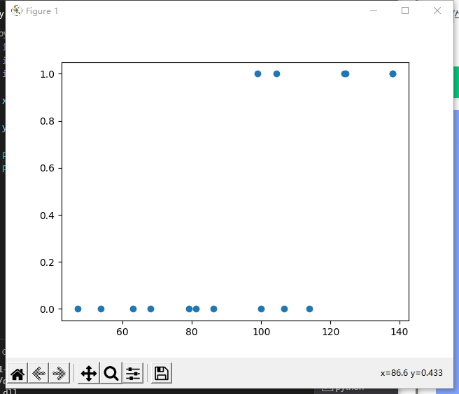
- 类别只有0和1两种
11.2.4.2 数据处理
x_train = x - np.mean(x)
y_train = y

plt.scatter(x_train,y_train)
plt.show()
输出结果为:
- 可以看到, 这些点整体平移,这些点相对位置不变
11.2.4.3 设置超参数
learn_rate = 0.005
iter = 5
display_step = 1
11.2.4.4 设置模型变量初始值
np.random.seed(612)
w = tf.Variable(np.random.randn())
b = tf.Variable(np.random.randn())
11.2.4.5 训练模型
cross_train = []
acc_train = []

for i in range(0,iter+1):

    with tf.GradientTape() as tape:
        pred_train = 1/(1+tf.exp(-w*x_train+b))
        Loss_train = -tf.reduce_mean(y_train*tf.math.log(pred_train)+(1-y_train)*tf.math.log(1-pred_train))
        Accuracy_train = tf.reduce_mean(tf.cast(tf.equal(tf.where(pred_train<0.5,0,1),y_train),tf.float32))

    cross_train.append(Loss_train)
    acc_train.append(Accuracy_train)

    dL_dw,dL_db = tape.gradient(Loss_train,[w,b])

    w.assign_sub(learn_rate*dL_dw)
    b.assign_sub(learn_rate*dL_db)

    if i % display_step == 0:
        print("i: %i, Train Loss: %f, Accuracy: %f" % (i,Loss_train,Accuracy_train))
输出结果为:
i: 0, Train Loss: 1.140986, Accuracy: 0.375000
i: 1, Train Loss: 0.703207, Accuracy: 0.625000
i: 2, Train Loss: 0.648479, Accuracy: 0.625000
i: 3, Train Loss: 0.631729, Accuracy: 0.687500
i: 4, Train Loss: 0.624276, Accuracy: 0.687500
i: 5, Train Loss: 0.620331, Accuracy: 0.750000
11.2.4.6 增加sigmoid曲线可视化输出
import tensorflow as tf
import numpy as np
import matplotlib.pyplot as plt

x = np.array([137.97,104.50,100.00,124.32,79.20,99.00,124.00,114.00,106.69,138.05,53.75,46.91,68.00,63.02,81.26,86.21])

y = np.array([1,1,0,1,0,1,1,0,0,1,0,0,0,0,0,0])

x_train = x - np.mean(x)
y_train = y

learn_rate = 0.005
iter = 5
display_step = 1

np.random.seed(612)
w = tf.Variable(np.random.randn())
b = tf.Variable(np.random.randn())

x_ = range(-80,80)
y_ = 1/(1+tf.exp(-(w*x_+b)))

plt.scatter(x_train,y_train)

plt.plot(x_,y_,c='r',linewidth=3)

cross_train = []
acc_train = []

for i in range(0,iter+1):

    with tf.GradientTape() as tape:
        pred_train = 1/(1+tf.exp(-w*x_train+b))
        Loss_train = -tf.reduce_mean(y_train*tf.math.log(pred_train)+(1-y_train)*tf.math.log(1-pred_train))
        Accuracy_train = tf.reduce_mean(tf.cast(tf.equal(tf.where(pred_train<0.5,0,1),y_train),tf.float32))

    cross_train.append(Loss_train)
    acc_train.append(Accuracy_train)

    dL_dw,dL_db = tape.gradient(Loss_train,[w,b])

    w.assign_sub(learn_rate*dL_dw)
    b.assign_sub(learn_rate*dL_db)

    if i % display_step == 0:
        print("i: %i, Train Loss: %f, Accuracy: %f" % (i,Loss_train,Accuracy_train))
        y_ = 1/(1+tf.exp(-(w*x_+b)))
        plt.plot(x_,y_)

plt.show()
输出结果为:
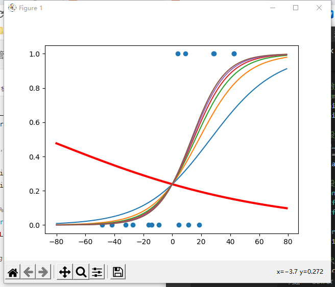
- 红色是使用初始参数时的sigmoid曲线,虽然看起来很离谱,但是恰好属于普通住宅的这10个样本的概率都在0.5以下,所以分类正确率为10/16
- 蓝色是第一次迭代结果
- 紫色是最后一次迭代的结果
- 在0-20之间,出现一段的重合,有一定的交集,所以这个区域中的点可能会出现分类错误,导致准确率无法达到100
- 第一次分类的结果,虽然正确率更大,但是从整体来看,还是经过更多次迭代之后更加合理
11.2.4.7 验证模型
x_test = [128.15,45.00,141.43,106.27,99.00,53.84,85.36,70.00,162.00,114.60]
pred_test = 1/(1+tf.exp(-(w*(x_test-np.mean(x))+b)))
y_test = tf.where(pred_test<0.5,0,1)
for i in range(len(x_test)):
    print(x_test[i],"\t",pred_test[i].numpy(),"\t",y_test[i].numpy(),"\t")
输出结果为:
128.15   0.84752923      1
45.0     0.003775026     0
141.43   0.94683856      1
106.27   0.4493811       0
99.0     0.30140132      0
53.84    0.008159011     0
85.36    0.11540905      0
70.0     0.032816157     0
162.0    0.99083763      1
114.6    0.62883806      1
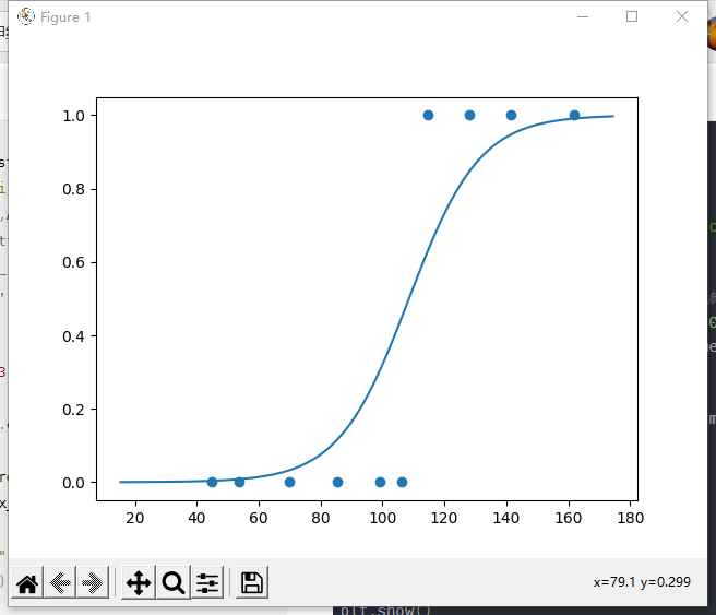
11.2.4.8 预测值的sigmoid曲线和散点图
import tensorflow as tf
import numpy as np
import matplotlib.pyplot as plt

x = np.array([137.97,104.50,100.00,124.32,79.20,99.00,124.00,114.00,106.69,138.05,53.75,46.91,68.00,63.02,81.26,86.21])

y = np.array([1,1,0,1,0,1,1,0,0,1,0,0,0,0,0,0])

x_train = x - np.mean(x)
y_train = y

learn_rate = 0.005
iter = 5
display_step = 1

np.random.seed(612)
w = tf.Variable(np.random.randn())
b = tf.Variable(np.random.randn())

cross_train = []
acc_train = []

for i in range(0,iter+1):

    with tf.GradientTape() as tape:
        pred_train = 1/(1+tf.exp(-w*x_train+b))
        Loss_train = -tf.reduce_mean(y_train*tf.math.log(pred_train)+(1-y_train)*tf.math.log(1-pred_train))
        Accuracy_train = tf.reduce_mean(tf.cast(tf.equal(tf.where(pred_train<0.5,0,1),y_train),tf.float32))

    cross_train.append(Loss_train)
    acc_train.append(Accuracy_train)

    dL_dw,dL_db = tape.gradient(Loss_train,[w,b])

    w.assign_sub(learn_rate*dL_dw)
    b.assign_sub(learn_rate*dL_db)

    if i % display_step == 0:
        print("i: %i, Train Loss: %f, Accuracy: %f" % (i,Loss_train,Accuracy_train))

x_test = [128.15,45.00,141.43,106.27,99.00,53.84,85.36,70.00,162.00,114.60]
pred_test = 1/(1+tf.exp(-(w*(x_test-np.mean(x))+b)))
y_test = tf.where(pred_test<0.5,0,1)
for i in range(len(x_test)):
    print(x_test[i],"\t",pred_test[i].numpy(),"\t",y_test[i].numpy(),"\t")

plt.scatter(x_test,y_test)

x_ = range(-80,80)
y_ = 1/(1+tf.exp(-(w*x_+b)))
plt.plot(x_+np.mean(x),y_)

plt.show()
输出结果为:
11.3 线性分类器(Linear Classifier)
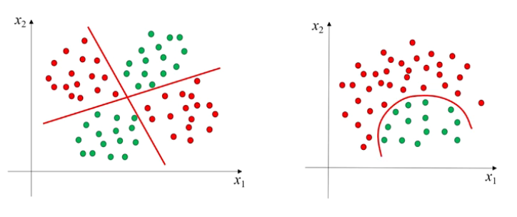
11.3.1 决策边界-线性可分
- 二维空间中的数据集,如果可以被一条直线分为两类,我们称之为 线性可分数据集,这条直线就是一个 线性分类器
- 在 三维空间中,如果数据集线性可分,是指被一个平面分为两类
- 在 一维空间中,所有的点都在一条直线上,线性可分可以理解为可以被一个点分开
- 这里的,分类直线、平面、点被称为 决策边界
- 一个m维数据集,
如果可以被一个超平面一分为二,那么这个数据集就是线性可分的,这个超平面就是决策边界
; 11.3.2 线性不可分
- 线性不可分:样本得两条直线分开,或者一条曲线分开
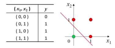
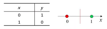
11.3.3 逻辑运算
11.3.3.1 线性可分-与、或、非
- 在逻辑运算中,与&、或|、非!都是线性可分的
- 显然可以通过训练得到对应的分类器,并且一定收敛
- 或运算
- 非运算
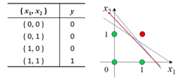
; 11.3.3.2 线性不可分-异或
- 异或运算,也可以看作是按类加运算
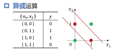
- 显然,要分开它,最少得两条直线
11.4 实例:实现多元逻辑回归
11.4.1 实现多元逻辑回归
11.4.1.1 鸢尾花数据集(iris)再次介绍
- 在这里,使用逻辑回归实现对鸢尾花(iris)的分类
-
Iris数据集
-
150个样本
- 4个属性:花萼长度(Sepal Length)、花萼宽度(Sepal Width)、花瓣长度(Petal Length)、花瓣宽度(Petal Width)
- 1个标签:山鸢尾(Setosa)、变色鸢尾(Versicolour)、维吉尼亚鸢尾(Virginica)
-
属性两两可视化后的结果为:
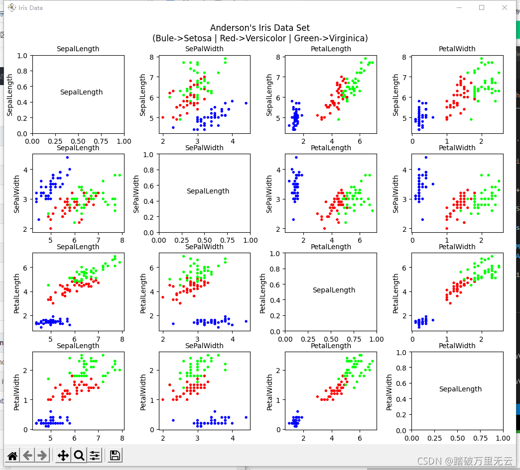
山鸢尾(蓝色)、变色鸢尾(红色)、维吉尼亚鸢尾(绿色) -
蓝色的与其他两个差别大,选择任何两个都可以区分开;所以选择蓝色(山鸢尾)的和红色(变色鸢尾)两种鸢尾花,花萼长度和花萼宽度两种属性,通过逻辑回归实现对他们的分类
- 了解鸢尾花数据集的具体使用方法可以参考【神经网络与深度学习-TensorFlow实践】-中国大学MOOC课程(六)(Matplotlib数据可视化))中的6.5节
; 11.4.1.2 实现多元逻辑回归
11.4.1.2.1 加载数据
import tensorflow as tf
import pandas as pd
import numpy as np
import matplotlib as mpl
import matplotlib.pyplot as plt

TRAIN_URL = "http://download.tensorflow.org/data/iris_training.csv"
train_path = tf.keras.utils.get_file(TRAIN_URL.split('/')[-1],TRAIN_URL)

df_iris = pd.read_csv(train_path,header=0)
11.4.1.2.2 处理数据
11.4.1.2.2.1 自己定义色彩方案mpl.colors.ListedColormap()
11.4.1.2.2.2 无须归一化,只需中心化
iris= np.array(df_iris)

train_x = iris[:,0:2]
train_y = iris[:,4]

x_train = train_x[train_y < 2]
y_train = train_y[train_y < 2]

num = len(x_train)

x_train = x_train - np.mean(x_train,axis= 0)

x0_train = np.ones(num).reshape(-1,1)
X = tf.cast(tf.concat((x0_train,x_train),axis=1),tf.float32)
Y = tf.cast(y_train.reshape(-1,1),tf.float32)
处理结果为:
- 可以看到中心化之后,样本点被平移,样本点的横坐标和纵坐标都是0
11.4.1.2.3 设置超参数
learn_rate = 0.2
iter = 120
display_step = 30
11.4.1.2.4 设置模型参数初始值
np.random.seed(612)
W = tf.Variable(np.random.randn(3,1),dtype=tf.float32)
11.4.1.2.5 训练模型
ce = []
acc = []

for i in range(0,iter+1):
    with tf.GradientTape() as tape:
        PRED = 1/(1+tf.exp(-tf.matmul(X,W)))
        Loss = -tf.reduce_mean(Y*tf.math.log(PRED)+(1-Y)*tf.math.log(1-PRED))

    accuracy = tf.reduce_mean(tf.cast(tf.equal(tf.where(PRED.numpy()<0.5,0.,1.),Y),tf.float32))
    ce.append(Loss)
    acc.append(accuracy)

    dL_dW = tape.gradient(Loss,W)
    W.assign_sub(learn_rate*dL_dW)

    if i % display_step ==0:
        print("i: %i, Acc: %f, Loss: %f" % (i,accuracy,Loss))
输出结果为:
i: 0, Acc: 0.230769, Loss: 0.994269
i: 30, Acc: 0.961538, Loss: 0.481892
i: 60, Acc: 0.987179, Loss: 0.319128
i: 90, Acc: 0.987179, Loss: 0.246626
i: 120, Acc: 1.000000, Loss: 0.204982
11.4.1.2.6 代码汇总(包含前五个步骤)
import tensorflow as tf
import pandas as pd
import numpy as np
import matplotlib as mpl
import matplotlib.pyplot as plt

TRAIN_URL = "http://download.tensorflow.org/data/iris_training.csv"
train_path = tf.keras.utils.get_file(TRAIN_URL.split('/')[-1],TRAIN_URL)

df_iris = pd.read_csv(train_path,header=0)

iris= np.array(df_iris)

train_x = iris[:,0:2]
train_y = iris[:,4]

x_train = train_x[train_y < 2]
y_train = train_y[train_y < 2]

num = len(x_train)

x_train = x_train - np.mean(x_train,axis= 0)

x0_train = np.ones(num).reshape(-1,1)
X = tf.cast(tf.concat((x0_train,x_train),axis=1),tf.float32)
Y = tf.cast(y_train.reshape(-1,1),tf.float32)

learn_rate = 0.2
iter = 120
display_step = 30

np.random.seed(612)
W = tf.Variable(np.random.randn(3,1),dtype=tf.float32)

ce = []
acc = []

for i in range(0,iter+1):
    with tf.GradientTape() as tape:
        PRED = 1/(1+tf.exp(-tf.matmul(X,W)))
        Loss = -tf.reduce_mean(Y*tf.math.log(PRED)+(1-Y)*tf.math.log(1-PRED))

    accuracy = tf.reduce_mean(tf.cast(tf.equal(tf.where(PRED.numpy()<0.5,0.,1.),Y),tf.float32))
    ce.append(Loss)
    acc.append(accuracy)

    dL_dW = tape.gradient(Loss,W)
    W.assign_sub(learn_rate*dL_dW)

    if i % display_step ==0:
        print("i: %i, Acc: %f, Loss: %f" % (i,accuracy,Loss))
11.4.1.2.6 可视化
11.4.1.2.6.1 绘制损失和准确率变化曲线
plt.figure(figsize=(5,3))
plt.plot(ce,c='b',label="Loss")
plt.plot(acc,c='r',label="acc")
plt.legend()
plt.show()
输出结果为:
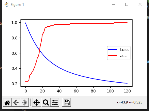
- 损失一直单调下降,所以损失下降曲线很光滑
- 而准确率上升到一定的数值之后,有时候会停留在某个时间一段时间,因此呈现出台阶上升的趋势
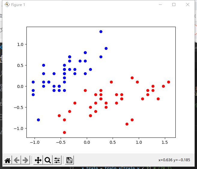
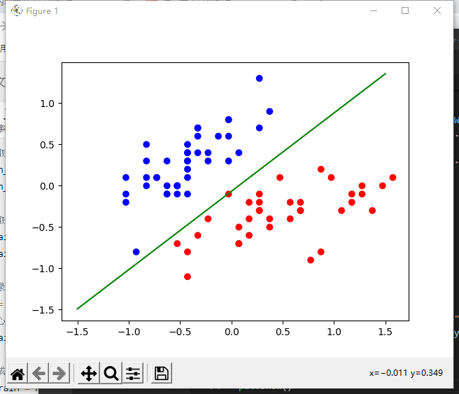
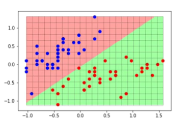
11.4.1.2.6.2 绘制决策边界
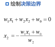
cm_pt = mpl.colors.ListedColormap(["blue","red"])
plt.scatter(x_train[:,0],x_train[:,1],c=y_train,cmap=cm_pt)
x_ = [-1.5,1.5]
y_ = -(W[1]*x_+W[0])/W[2]
plt.plot(x_,y_,c='g')
plt.show()
输出结果为:
11.4.1.2.6.3 在训练过程中绘制决策边界*
import tensorflow as tf
import pandas as pd
import numpy as np
import matplotlib as mpl
import matplotlib.pyplot as plt

TRAIN_URL = "http://download.tensorflow.org/data/iris_training.csv"
train_path = tf.keras.utils.get_file(TRAIN_URL.split('/')[-1],TRAIN_URL)

df_iris = pd.read_csv(train_path,header=0)

iris= np.array(df_iris)

train_x = iris[:,0:2]
train_y = iris[:,4]

x_train = train_x[train_y < 2]
y_train = train_y[train_y < 2]

num = len(x_train)

x_train = x_train - np.mean(x_train,axis= 0)

x0_train = np.ones(num).reshape(-1,1)
X = tf.cast(tf.concat((x0_train,x_train),axis=1),tf.float32)
Y = tf.cast(y_train.reshape(-1,1),tf.float32)

learn_rate = 0.2
iter = 120
display_step = 30

np.random.seed(612)
W = tf.Variable(np.random.randn(3,1),dtype=tf.float32)

cm_pt = mpl.colors.ListedColormap(["blue","red"])

x_ = [-1.5,1.5]
y_ = -(W[0]+W[1]*x_)/W[2]

plt.scatter(x_train[:,0],x_train[:,1],c=y_train,cmap=cm_pt)
plt.plot(x_,y_,c='r',linewidth=3)
plt.xlim([-1.5,1.5])
plt.ylim([-1.5,1.5])

ce = []
acc = []

for i in range(0,iter+1):
    with tf.GradientTape() as tape:
        PRED = 1/(1+tf.exp(-tf.matmul(X,W)))
        Loss = -tf.reduce_mean(Y*tf.math.log(PRED)+(1-Y)*tf.math.log(1-PRED))

    accuracy = tf.reduce_mean(tf.cast(tf.equal(tf.where(PRED.numpy()<0.5,0.,1.),Y),tf.float32))
    ce.append(Loss)
    acc.append(accuracy)

    dL_dW = tape.gradient(Loss,W)
    W.assign_sub(learn_rate*dL_dW)

    if i % display_step ==0:
        print("i: %i, Acc: %f, Loss: %f" % (i,accuracy,Loss))
        y_ = -(W[0]+W[1]*x_)/W[2]
        plt.plot(x_,y_)

plt.show()
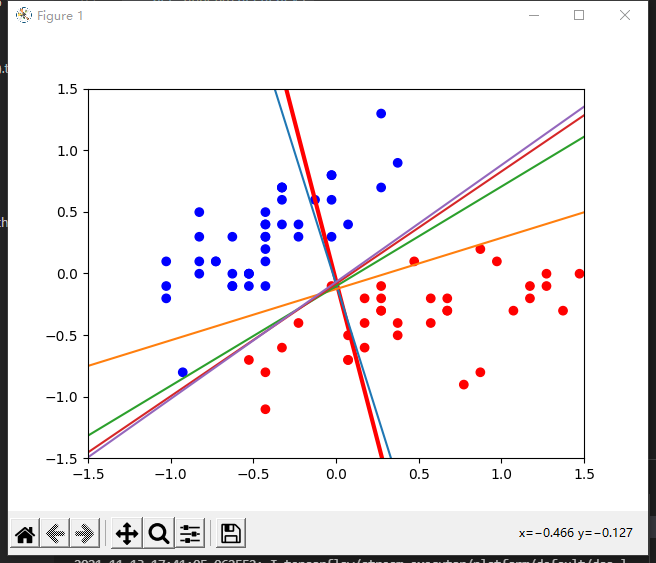
- 红色的是初始的,之后慢慢调增
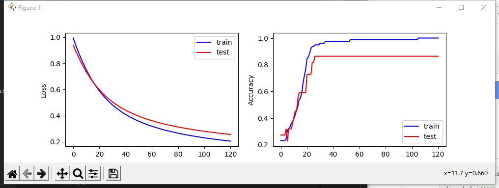
11.4.1.2.7 使用测试集
import tensorflow as tf
import pandas as pd
import numpy as np
import matplotlib as mpl
import matplotlib.pyplot as plt

TRAIN_URL = "http://download.tensorflow.org/data/iris_training.csv"
TEST_URL = "http://download.tensorflow.org/data/iris_test.csv"
train_path = tf.keras.utils.get_file(TRAIN_URL.split('/')[-1],TRAIN_URL)
test_path = tf.keras.utils.get_file(TEST_URL.split('/')[-1],TEST_URL)

df_iris_train = pd.read_csv(train_path,header=0)
df_iris_test =  pd.read_csv(test_path,header=0)

iris_train= np.array(df_iris_train)
iris_test= np.array(df_iris_test)

train_x = iris_train[:,0:2]
train_y = iris_train[:,4]

test_x = iris_test[:,0:2]
test_y = iris_test[:,4]

x_train = train_x[train_y < 2]
y_train = train_y[train_y < 2]

x_test = test_x[test_y < 2]
y_test = test_y[test_y < 2]

num_train = len(x_train)
num_test = len(x_test)

x_train = x_train - np.mean(x_train,axis= 0)
x_test = x_test - np.mean(x_test,axis=0)

x0_train = np.ones(num_train).reshape(-1,1)
X_train = tf.cast(tf.concat((x0_train,x_train),axis=1),tf.float32)
Y_train = tf.cast(y_train.reshape(-1,1),tf.float32)

x0_test = np.ones(num_test).reshape(-1,1)
X_test = tf.cast(tf.concat((x0_test,x_test),axis=1),dtype=tf.float32)
Y_test = tf.cast(y_test.reshape(-1,1),dtype=tf.float32)

learn_rate = 0.2
iter = 120
display_step = 30

np.random.seed(612)
W = tf.Variable(np.random.randn(3,1),dtype=tf.float32)

cm_pt = mpl.colors.ListedColormap(["blue","red"])

x_ = [-1.5,1.5]
y_ = -(W[0]+W[1]*x_)/W[2]

ce_train = []
acc_train = []
ce_test = []
acc_test = []

for i in range(0,iter+1):
    with tf.GradientTape() as tape:
        PRED_train = 1/(1+tf.exp(-tf.matmul(X_train,W)))
        Loss_train = -tf.reduce_mean(Y_train*tf.math.log(PRED_train)+(1-Y_train)*tf.math.log(1-PRED_train))
        PRED_test = 1/(1+tf.exp(-tf.matmul(X_test,W)))
        Loss_test = -tf.reduce_mean(Y_test*tf.math.log(PRED_test)+(1-Y_test)*tf.math.log(1-PRED_test))

    accuracy_train = tf.reduce_mean(tf.cast(tf.equal(tf.where(PRED_train.numpy()<0.5,0.,1.),Y_train),tf.float32))
    accuracy_test = tf.reduce_mean(tf.cast(tf.equal(tf.where(PRED_test.numpy()<0.5,0.,1.),Y_test),tf.float32))

    ce_train.append(Loss_train)
    acc_train.append(accuracy_train)
    ce_test.append(Loss_test)
    acc_test.append(accuracy_test)

    dL_dW = tape.gradient(Loss_train,W)
    W.assign_sub(learn_rate*dL_dW)

    if i % display_step ==0:
        print("i: %i, TrainAcc: %f, TrainLoss: %f, TestAcc: %f, TestLoss: %f" % (i,accuracy_train,Loss_train,accuracy_test,Loss_test))

plt.figure(figsize=(10,3))

plt.subplot(121)
plt.plot(ce_train,c='b',label="train")
plt.plot(ce_test,c='r',label="test")
plt.ylabel("Loss")
plt.legend()

plt.subplot(122)
plt.plot(acc_train,c='b',label="train")
plt.plot(acc_test,c='r',label="test")
plt.ylabel("Accuracy")

plt.legend()
plt.show()
输出结果为:
i: 0, TrainAcc: 0.230769, TrainLoss: 0.994269, TestAcc: 0.272727, TestLoss: 0.939684
i: 30, TrainAcc: 0.961538, TrainLoss: 0.481892, TestAcc: 0.863636, TestLoss: 0.505456
i: 60, TrainAcc: 0.987179, TrainLoss: 0.319128, TestAcc: 0.863636, TestLoss: 0.362112
i: 90, TrainAcc: 0.987179, TrainLoss: 0.246626, TestAcc: 0.863636, TestLoss: 0.295611
i: 120, TrainAcc: 1.000000, TrainLoss: 0.204982, TestAcc: 0.863636, TestLoss: 0.256212
11.4.2 绘制分类图
; 11.4.2.1 生成网格坐标矩阵np.meshgrid()
X,Y = np.meshgrid(x,y)
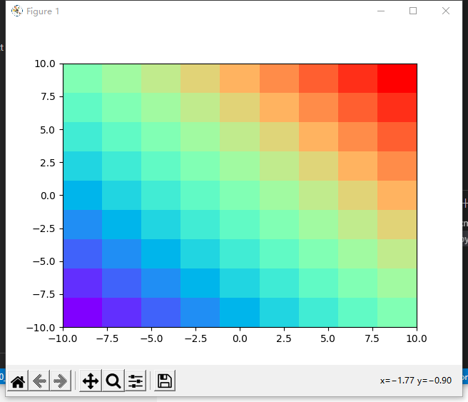
11.4.2.2 填充网格 plt.pcolomesh()
11.4.2.2.1 rainbow色彩方案
plt.pcolomesh(X,Y,Z,cmap)
- 前两个参数:X和Y确定网格位置
- 第三个参数:Z决定网格的颜色
- 第四个参数:cmap指定所使用的颜色方案
- 可以使用plt.contourf()函数代替plt.pcolomesh()函数
import tensorflow as tf
import numpy as np
import matplotlib as mpl
import matplotlib.pyplot as plt

n = 10
x = np.linspace(-10,10,n)
y = np.linspace(-10,10,n)
X,Y = np.meshgrid(x,y)
Z = X+Y
plt.pcolormesh(X,Y,Z,cmap="rainbow")

plt.show()
输出结果为:
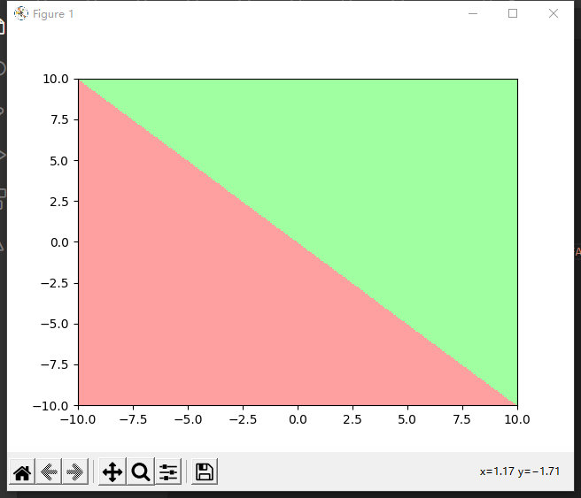
11.4.2.2.2 自己定义的色彩方案
- 如果定义了两种颜色,就平均按照颜色值划分两类,如果是三种颜色,就划分为三个区域
import tensorflow as tf
import numpy as np
import matplotlib as mpl
import matplotlib.pyplot as plt

n = 200
x = np.linspace(-10,10,n)
y = np.linspace(-10,10,n)
X,Y = np.meshgrid(x,y)
Z = X+Y
cm_bg = mpl.colors.ListedColormap(["#FFA0A0","#A0FFA0"])
plt.pcolormesh(X,Y,Z,cmap=cm_bg)

plt.show()
输出结果为:
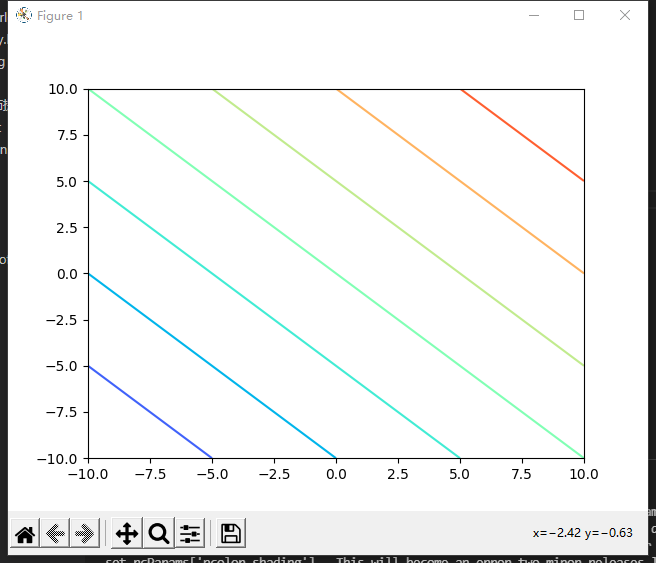
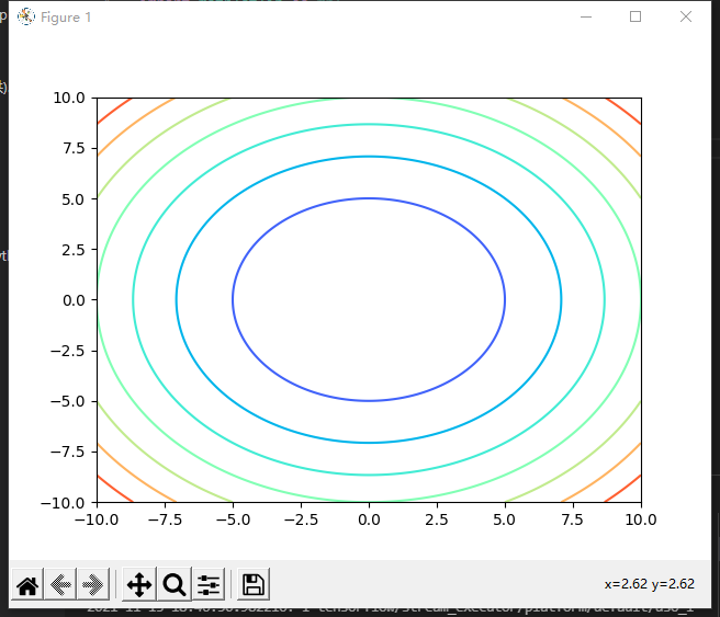
11.4.2.3 绘制轮廓线plt.contour()
- plt.contour():根据类的取值绘制出相同取值的边界
- 可以理解为三维模型的等高线
import tensorflow as tf
import numpy as np
import matplotlib as mpl
import matplotlib.pyplot as plt

n = 200
x = np.linspace(-10,10,n)
y = np.linspace(-10,10,n)
X,Y = np.meshgrid(x,y)
Z = X+Y

plt.contour(X,Y,Z,cmap="rainbow")

plt.show()
输出结果为:
修改为
Z = X**2+Y**2
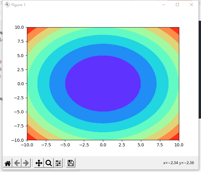
11.4.2.3.1 给轮廓线之间填充颜色plt.contourf(X,Y,Z,a,cmap)
- 填充分区
plt.contourf(X,Y,Z,a,cmap)
- 前两个参数:X和Y确定网格位置
- 第三个参数:Z决定网格的颜色
- 第四个参数:a,指定颜色细分的数量
- 第五个参数:cmap指定所使用的颜色方案
- 可以使用plt.contourf()函数代替plt.pcolomesh()函数
import tensorflow as tf
import numpy as np
import matplotlib as mpl
import matplotlib.pyplot as plt

n = 200
x = np.linspace(-10,10,n)
y = np.linspace(-10,10,n)
X,Y = np.meshgrid(x,y)
Z = X**2+Y**2

plt.contourf(X,Y,Z,cmap="rainbow")

plt.show()
输出结果为:
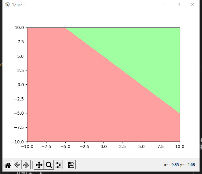
11.4.2.4 绘制分类图例子
import tensorflow as tf
import numpy as np
import matplotlib as mpl
import matplotlib.pyplot as plt

n = 200
x = np.linspace(-10,10,n)
y = np.linspace(-10,10,n)
X,Y = np.meshgrid(x,y)
Z = X+Y

cm_bg = mpl.colors.ListedColormap(["#FFA0A0","#A0FFA0"])
Z = tf.where(Z<5,0,1)
plt.contourf(X,Y,Z,cmap=cm_bg)

plt.show()
输出结果为:
11.4.2.5 根据鸢尾花分类模型,绘制训练集和测试集分类图
import tensorflow as tf
import pandas as pd
import numpy as np
import matplotlib as mpl
import matplotlib.pyplot as plt
TRAIN_URL = "http://download.tensorflow.org/data/iris_training.csv"
TEST_URL = "http://download.tensorflow.org/data/iris_test.csv"
train_path = tf.keras.utils.get_file(TRAIN_URL.split('/')[-1],TRAIN_URL)
test_path = tf.keras.utils.get_file(TEST_URL.split('/')[-1],TEST_URL)
df_iris_train = pd.read_csv(train_path,header=0)
df_iris_test = pd.read_csv(test_path,header=0)
iris_train= np.array(df_iris_train)
iris_test= np.array(df_iris_test)
train_x = iris_train[:,0:2]
train_y = iris_train[:,4]
test_x = iris_test[:,0:2]
test_y = iris_test[:,4]
x_train = train_x[train_y < 2]
y_train = train_y[train_y < 2]
x_test = test_x[test_y < 2]
y_test = test_y[test_y < 2]
num_train = len(x_train)
num_test = len(x_test)
x_train = x_train - np.mean(x_train,axis= 0)
x_test = x_test - np.mean(x_test,axis=0)
x0_train = np.ones(num_train).reshape(-1,1)
X_train = tf.cast(tf.concat((x0_train,x_train),axis=1),tf.float32)
Y_train = tf.cast(y_train.reshape(-1,1),tf.float32)
x0_test = np.ones(num_test).reshape(-1,1)
X_test = tf.cast(tf.concat((x0_test,x_test),axis=1),dtype=tf.float32)
Y_test = tf.cast(y_test.reshape(-1,1),dtype=tf.float32)
learn_rate = 0.2
iter = 120
display_step = 30
np.random.seed(612)
W = tf.Variable(np.random.randn(3,1),dtype=tf.float32)
cm_pt = mpl.colors.ListedColormap(["blue","red"])
x_ = [-1.5,1.5]
y_ = -(W[0]+W[1]*x_)/W[2]
ce_train = []
acc_train = []
ce_test = []
acc_test = []
for i in range(0,iter+1):
with tf.GradientTape() as tape:
PRED_train = 1/(1+tf.exp(-tf.matmul(X_train,W)))
Loss_train = -tf.reduce_mean(Y_train*tf.math.log(PRED_train)+(1-Y_train)*tf.math.log(1-PRED_train))
PRED_test = 1/(1+tf.exp(-tf.matmul(X_test,W)))
Loss_test = -tf.reduce_mean(Y_test*tf.math.log(PRED_test)+(1-Y_test)*tf.math.log(1-PRED_test))
accuracy_train = tf.reduce_mean(tf.cast(tf.equal(tf.where(PRED_train.numpy()<0.5,0.,1.),Y_train),tf.float32))
accuracy_test = tf.reduce_mean(tf.cast(tf.equal(tf.where(PRED_test.numpy()<0.5,0.,1.),Y_test),tf.float32))
ce_train.append(Loss_train)
acc_train.append(accuracy_train)
ce_test.append(Loss_test)
acc_test.append(accuracy_test)
dL_dW = tape.gradient(Loss_train,W)
W.assign_sub(learn_rate*dL_dW)
if i % display_step ==0:
print("i: %i, TrainAcc: %f, TrainLoss: %f, TestAcc: %f, TestLoss: %f" % (i,accuracy_train,Loss_train,accuracy_test,Loss_test))
cm_pt = mpl.colors.ListedColormap(["blue","red"])
cm_bg = mpl.colors.ListedColormap(["#FFA0A0","#A0FFA0"])
plt.rcParams['font.sans-serif']="SimHei"
plt.figure(figsize=(15,5))
plt.subplot(121)
M = 300
x1_min,x2_min = x_train.min(axis=0)
x1_max,x2_max = x_train.max(axis=0)
t1 = np.linspace(x1_min,x1_max,M)
t2 = np.linspace(x2_min,x2_max,M)
m1,m2 = np.meshgrid(t1,t2)
m0 = np.ones(M*M)
X_mesh = tf.cast(np.stack((m0,m1.reshape(-1),m2.reshape(-1)),axis=1),dtype=tf.float32)
Y_mesh = tf.cast(1/(1+tf.exp(-tf.matmul(X_mesh,W))),dtype=tf.float32)
Y_mesh = tf.where(Y_mesh<0.5,0,1)
n = tf.reshape(Y_mesh,m1.shape)
plt.pcolormesh(m1,m2,n,cmap=cm_bg)
plt.scatter(x_train[:,0],x_train[:,1],c=y_train,cmap=cm_pt)
plt.title("训练集分类图",fontsize = 14)
plt.legend()
plt.subplot(122)
M = 300
x1_min,x2_min = x_test.min(axis=0)
x1_max,x2_max = x_test.max(axis=0)
t1 = np.linspace(x1_min,x1_max,M)
t2 = np.linspace(x2_min,x2_max,M)
m1,m2 = np.meshgrid(t1,t2)
m0 = np.ones(M*M)
X_mesh = tf.cast(np.stack((m0,m1.reshape(-1),m2.reshape(-1)),axis=1),dtype=tf.float32)
Y_mesh = tf.cast(1/(1+tf.exp(-tf.matmul(X_mesh,W))),dtype=tf.float32)
Y_mesh = tf.where(Y_mesh<0.5,0,1)
n = tf.reshape(Y_mesh,m1.shape)
plt.pcolormesh(m1,m2,n,cmap=cm_bg)
plt.scatter(x_test[:,0],x_test[:,1],c=y_test,cmap=cm_pt)
plt.title("测试集分类图",fontsize = 14)
plt.legend()
plt.show()
x1_max,x2_max = x_train.max(axis=0)
t1 = np.linspace(x1_min,x1_max,M)
t2 = np.linspace(x2_min,x2_max,M)

shgrid(t1,t2)
m0 = np.ones(M*M)
X_mesh = tf.cast(np.stack((m0,m1.reshape(-1),m2.reshape(-1)),axis=1),dtype=tf.float32)
Y_mesh = tf.cast(1/(1+tf.exp(-tf.matmul(X_mesh,W))),dtype=tf.float32)
Y_mesh = tf.where(Y_mesh<0.5,0,1)
n = tf.reshape(Y_mesh,m1.shape)
plt.pcolormesh(m1,m2,n,cmap=cm_bg)
plt.scatter(x_train[:,0],x_train[:,1],c=y_train,cmap=cm_pt)
plt.subplot(122)
M = 300
x1_min,x2_min = x_test.min(axis=0)
x1_max,x2_max = x_test.max(axis=0)
t1 = np.linspace(x1_min,x1_max,M)
t2 = np.linspace(x2_min,x2_max,M)
m1,m2 = np.meshgrid(t1,t2)
m0 = np.ones(M*M)
X_mesh = tf.cast(np.stack((m0,m1.reshape(-1),m2.reshape(-1)),axis=1),dtype=tf.float32)
Y_mesh = tf.cast(1/(1+tf.exp(-tf.matmul(X_mesh,W))),dtype=tf.float32)
Y_mesh = tf.where(Y_mesh<0.5,0,1)
n = tf.reshape(Y_mesh,m1.shape)
plt.pcolormesh(m1,m2,n,cmap=cm_bg)
plt.scatter(x_test[:,0],x_test[:,1],c=y_test,cmap=cm_pt)
plt.show()
输出结果为:
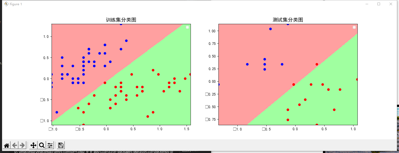
- 测试集上看着有两个分类错误,其实是三个,因为测试集里面有两个重合点
11.4.2.5 使用定义函数借鉴上一节代码
讨论【11.4】绘制测试集分类图
课程编程实例中,有很多代码是重复的,是否可以通过函数来实现代码复用?同学们尝试一下,并在讨论区分享关键代码,大家共同学习。
import tensorflow as tf
import numpy as np
import matplotlib as mpl
import matplotlib.pyplot as plt
import pandas as pd
from numpy.lib.function_base import disp

def preparedData(URL):
    path=tf.keras.utils.get_file(URL.split('/')[-1],URL)
    df_iris=pd.read_csv(path,header=0)
    iris=np.array(df_iris)
    _x=iris[:,0:2]
    _y=iris[:,4]
    x=_x[_y<2]
    y=_y[_y<2]
    num=len(x)
    X,Y,x=dataCentralize(x,y,num)
    return X,Y,x,y

def dataCentralize(x,y,num):
    x=x-np.mean(x,axis=0)
    x0=np.ones(num).reshape(-1,1)
    X=tf.cast(tf.concat((x0,x),axis=1),tf.float32)
    Y=tf.cast(y.reshape(-1,1),tf.float32)
    return X,Y,x

def getDerivate(X,Y,W,ce,acc,flag):
    with tf.GradientTape() as tape:
        PRED=1/(1+tf.exp(-tf.matmul(X,W)))
        Loss=-tf.reduce_mean(Y*tf.math.log(PRED)+(1-Y)*tf.math.log(1-PRED))
        accuracy=tf.reduce_mean(tf.cast(tf.equal(tf.where(PRED.numpy()<0.5,0.,1.),Y),tf.float32))
        ce.append(Loss)

        acc.append(accuracy)
        if  flag==1:
            dL_dW=tape.gradient(Loss,W)
            W.assign_sub(learn_rate*dL_dW)
    return ce,acc,W

def mapping(x,y):
    M=300
    x1_min,x2_min=x.min(axis=0)
    x1_max,x2_max=x.max(axis=0)
    t1=np.linspace(x1_min,x1_max,M)
    t2=np.linspace(x2_min,x2_max,M)
    m1,m2=np.meshgrid(t1,t2)
    m0=np.ones(M*M)
    X_mesh=tf.cast(np.stack((m0,m1.reshape(-1),m2.reshape(-1)),axis=1),dtype=tf.float32)
    Y_mesh=tf.cast(1/(1+tf.exp(-tf.matmul(X_mesh,W))),dtype=tf.float32)
    Y_mesh=tf.where(Y_mesh<0.5,0,1)
    n=tf.reshape(Y_mesh,m1.shape)
    cm_pt=mpl.colors.ListedColormap(["blue","red"])
    cm_bg=mpl.colors.ListedColormap(["#FFA0A0","#A0FFA0"])
    plt.pcolormesh(m1,m2,n,cmap=cm_bg)
    plt.scatter(x[:,0],x[:,1],c=y,cmap=cm_pt)
    plt.show()

TRAIN_URL="https://download.tensorflow.org/data/iris_training.csv"
TEST_URL="https://download.tensorflow.org/data/iris_test.csv"
X_train,Y_train,x_train,y_train=preparedData(TRAIN_URL)
X_test,Y_test,x_test,y_test=preparedData(TEST_URL)

learn_rate=0.2
iter=120
display_step=30

np.random.seed(612)
W=tf.Variable(np.random.randn(3,1),dtype=tf.float32)

ce_train=[]
acc_train=[]
ce_test=[]
acc_test=[]

for i in range(0,iter+1):
    acc_train,ce_train,W=getDerivate(X_train,Y_train,W,ce_train,acc_train,1)
    acc_test,ce_test,W=getDerivate(X_train,Y_train,W,ce_train,acc_train,1)
    if i % display_step==0:
        print("i:%i\tAcc:%f\tLoss:%f\tAcc_test:%f\tLoss_test:%f"%(i,acc_train[i],ce_train[i],acc_test[i],ce_test[i]))

mapping(x_test,y_test)
输出结果为:
i:0     Acc:0.994269    Loss:0.230769   Acc_test:0.230769       Loss_test:0.994269
i:30    Acc:0.961538    Loss:0.481892   Acc_test:0.481892       Loss_test:0.961538
i:60    Acc:0.319128    Loss:0.987179   Acc_test:0.987179       Loss_test:0.319128
i:90    Acc:0.987179    Loss:0.246626   Acc_test:0.246626       Loss_test:0.987179
i:120   Acc:0.204982    Loss:1.000000   Acc_test:1.000000       Loss_test:0.204982
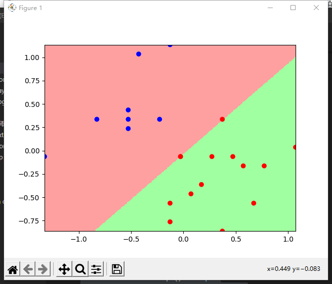
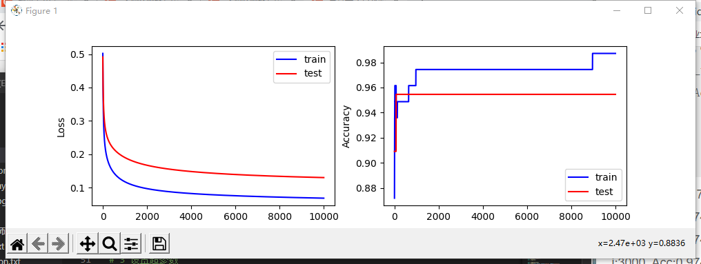
11.4.2.6 使用四种属性区分变色鸢尾和维吉尼亚鸢尾
鸢尾花数据集中,有四个属性(花瓣长度、花瓣宽度、花萼长度、花萼宽度),课程中只是给出了两种属性组合的情况,如果采用三种或者四种属性去训练模型,能否把变色鸢尾和维吉尼亚鸢尾完全区分开呢?请简要说明一下你用的哪几种属性并在讨论区晒出你的程序结果。
import tensorflow as tf
import pandas as pd
import numpy as np
import matplotlib as mpl
import matplotlib.pyplot as plt

TRAIN_URL = "http://download.tensorflow.org/data/iris_training.csv"
TEST_URL = "http://download.tensorflow.org/data/iris_test.csv"
train_path = tf.keras.utils.get_file(TRAIN_URL.split('/')[-1],TRAIN_URL)
test_path = tf.keras.utils.get_file(TEST_URL.split('/')[-1],TEST_URL)

df_iris_train = pd.read_csv(train_path,header=0)
df_iris_test =  pd.read_csv(test_path,header=0)

iris_train= np.array(df_iris_train)
iris_test= np.array(df_iris_test)

train_x = iris_train[:,0:4]
train_y = iris_train[:,4]

test_x = iris_test[:,0:4]
test_y = iris_test[:,4]

x_train = train_x[train_y > 0]
y_train = train_y[train_y > 0]-1

x_test = test_x[test_y > 0]
y_test = test_y[test_y > 0]-1

num_train = len(x_train)
num_test = len(x_test)

x_train = x_train - np.mean(x_train,axis= 0)
x_test = x_test - np.mean(x_test,axis=0)

x0_train = np.ones(num_train).reshape(-1,1)
X_train = tf.cast(tf.concat((x0_train,x_train),axis=1),tf.float32)
Y_train = tf.cast(y_train.reshape(-1,1),tf.float32)

x0_test = np.ones(num_test).reshape(-1,1)
X_test = tf.cast(tf.concat((x0_test,x_test),axis=1),dtype=tf.float32)
Y_test = tf.cast(y_test.reshape(-1,1),dtype=tf.float32)

learn_rate = 0.135
iter = 10000
display_step = 1000

np.random.seed(612)
W = tf.Variable(np.random.randn(5,1),dtype=tf.float32)

ce_train = []
acc_train = []
ce_test = []
acc_test = []

for i in range(0,iter+1):
    with tf.GradientTape() as tape:
        PRED_train = 1/(1+tf.exp(-tf.matmul(X_train,W)))
        Loss_train = -tf.reduce_mean(Y_train*tf.math.log(PRED_train)+(1-Y_train)*tf.math.log(1-PRED_train))
        PRED_test = 1/(1+tf.exp(-tf.matmul(X_test,W)))
        Loss_test = -tf.reduce_mean(Y_test*tf.math.log(PRED_test)+(1-Y_test)*tf.math.log(1-PRED_test))

    accuracy_train = tf.reduce_mean(tf.cast(tf.equal(tf.where(PRED_train.numpy()<0.5,0.,1.),Y_train),tf.float32))
    accuracy_test = tf.reduce_mean(tf.cast(tf.equal(tf.where(PRED_test.numpy()<0.5,0.,1.),Y_test),tf.float32))

    ce_train.append(Loss_train)
    acc_train.append(accuracy_train)
    ce_test.append(Loss_test)
    acc_test.append(accuracy_test)

    dL_dW = tape.gradient(Loss_train,W)
    W.assign_sub(learn_rate*dL_dW)

    if i % display_step ==0:
        print("i: %i, TrainAcc: %f, TrainLoss: %f, TestAcc: %f, TestLoss: %f" % (i,accuracy_train,Loss_train,accuracy_test,Loss_test))

plt.figure(figsize=(10,3))
plt.subplot(121)
plt.plot(ce_train,color="blue",label="train")
plt.plot(ce_test,color="red",label="test")
plt.ylabel("Loss")
plt.legend()

plt.subplot(122)
plt.plot(acc_train,color="blue",label="train")
plt.plot(acc_test,color="red",label="test")
plt.ylabel("Accuracy")
plt.legend()

plt.show()
输出结果为:
i: 0, TrainAcc: 0.871795, TrainLoss: 0.502093, TestAcc: 0.909091, TestLoss: 0.491409
i: 1000, TrainAcc: 0.974359, TrainLoss: 0.117291, TestAcc: 0.954545, TestLoss: 0.189897
i: 2000, TrainAcc: 0.974359, TrainLoss: 0.096742, TestAcc: 0.954545, TestLoss: 0.166818
i: 3000, TrainAcc: 0.974359, TrainLoss: 0.087580, TestAcc: 0.954545, TestLoss: 0.155260
i: 4000, TrainAcc: 0.974359, TrainLoss: 0.082096, TestAcc: 0.954545, TestLoss: 0.148034
i: 5000, TrainAcc: 0.974359, TrainLoss: 0.078296, TestAcc: 0.954545, TestLoss: 0.142953
i: 6000, TrainAcc: 0.974359, TrainLoss: 0.075425, TestAcc: 0.954545, TestLoss: 0.139118
i: 7000, TrainAcc: 0.974359, TrainLoss: 0.073129, TestAcc: 0.954545, TestLoss: 0.136092
i: 8000, TrainAcc: 0.974359, TrainLoss: 0.071221, TestAcc: 0.954545, TestLoss: 0.133636
i: 9000, TrainAcc: 0.987179, TrainLoss: 0.069592, TestAcc: 0.954545, TestLoss: 0.131605
i: 10000, TrainAcc: 0.987179, TrainLoss: 0.068172, TestAcc: 0.954545, TestLoss: 0.129906
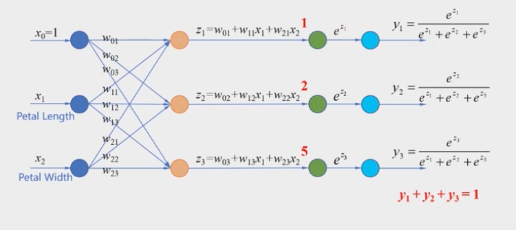
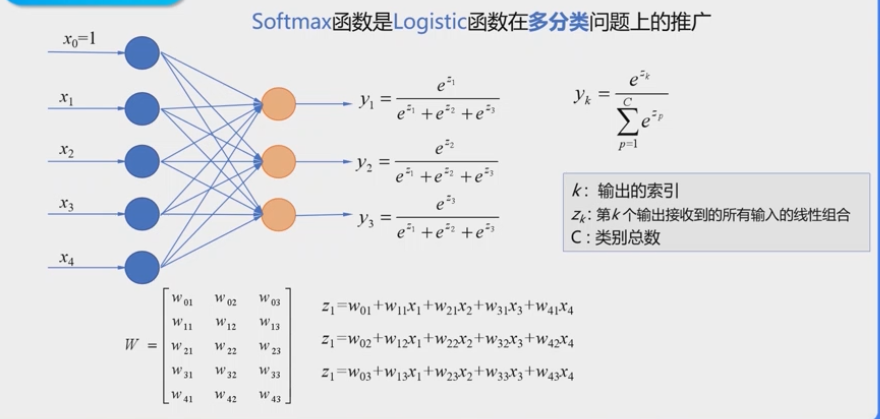
11.5 多分类问题
- 逻辑回归:二分类问题
- 多分类问题:把输入样本划分为多个类别
- 下面以鸢尾花为例,实现多分类类别
11.5.1 类别编码问题
- 自然顺序码
0 —— 山鸢尾(Setosa)
1 —— 变色鸢尾(Versicolour)
2 —— 维吉尼亚鸢尾(Virginica)
欧氏距离使得类别之间不平等,但是实际上类别之间应该是平等的 - 独热编码(One-Hot Encoding)
使非偏序关系的数据,取值不具有偏序性
到原点等距
(1,0,0) —— 山鸢尾(Setosa)
(0,1,0) —— 变色鸢尾(Versicolour)
(0,0,1) —— 维吉尼亚鸢尾(Virginica)
需要占用更多的空间,但是能够更加合理的表示数据之间的关系,可以有效的避免学习中的偏差 - 独热的 应用
离散的特征
多分类问题中的类别标签 - 独冷编码(One-Hot Encoding)
(0,1,1) —— 山鸢尾(Setosa)
(1,0,1) —— 变色鸢尾(Versicolour)
(1,1,0) —— 维吉尼亚鸢尾(Virginica)
11.5.2 实例,多分类问题
- 例:使用属性花瓣长度和花瓣宽度,构造分类器,能够识别3种类型的鸢尾花
- 互斥的多分类问题:每个样本只能够属于一个类别
鸢尾花的识别
手写数字的识别 - 标签:一个图片可以被打上多个标签,即一个样本可以同时属于多个类别
彩色图片
包括人物的图片
包括汽车的图片
户外图片
室内图片
; 11.6 实例:多分类问题
11.6.1 独热编码的实现
tf.one_hot(indices,depth)
- indices:一维数组/张量
- depth:编码深度,也就是分成几类
>>> import tensorflow as tf
>>> print(tf.__version__)
2.0.0
>>> import numpy as np
>>> a = [0,2,3,5]
>>> b = tf.one_hot(a,6)
>>> b
<tf.Tensor: id=9, shape=(4, 6), dtype=float32, numpy=
array([[1., 0., 0., 0., 0., 0.],
       [0., 0., 1., 0., 0., 0.],
       [0., 0., 0., 1., 0., 0.],
       [0., 0., 0., 0., 0., 1.]], dtype=float32)>
11.6.2 准确率的计算
>>> pred = np.array([[0.1,0.2,0.7],[0.1,0.7,0.2],[0.3,0.4,0.3]])

>>> y = np.array([2,1,0])

>>> y_onehot = np.array([[0,0,1],[0,1,0],[1,0,0]])

>>> tf.argmax(pred,axis=1)
<tf.Tensor: id=12, shape=(3,), dtype=int64, numpy=array([2, 1, 1], dtype=int64)>

>>> tf.equal(tf.argmax(pred,axis=1),y)
<tf.Tensor: id=17, shape=(3,), dtype=bool, numpy=array([ True,  True, False])>

>>> tf.cast(tf.equal(tf.argmax(pred,axis=1),y),tf.float32)
<tf.Tensor: id=23, shape=(3,), dtype=float32, numpy=array([1., 1., 0.], dtype=float32)>

>>> tf.reduce_mean(tf.cast(tf.equal(tf.argmax(pred,axis=1),y),tf.float32))
<tf.Tensor: id=39, shape=(), dtype=float32, numpy=0.6666667>
11.6.3 交叉熵损失函数的实现
代码接11.6.2
>>> -y_onehot*tf.math.log(pred)
<tf.Tensor: id=43, shape=(3, 3), dtype=float64, numpy=
array([[-0.        , -0.        ,  0.35667494],
       [-0.        ,  0.35667494, -0.        ],
       [ 1.2039728 , -0.        , -0.        ]])>

>>> -tf.reduce_sum(y_onehot*tf.math.log(pred))
<tf.Tensor: id=50, shape=(), dtype=float64, numpy=1.917322692203401>

>>> -tf.reduce_sum(y_onehot*tf.math.log(pred))/len(pred)
<tf.Tensor: id=59, shape=(), dtype=float64, numpy=0.6391075640678003>
>>> len(pred)
3
11.6.4 使用花瓣长度、花瓣宽度将三种鸢尾花区分开
11.6.4.0 修改动态分配显存
https://blog.csdn.net/qq_45954434/article/details/121236512
这里不修改显存分配我的就会报错,所以这里会默认修改动态显存分配
11.6.4.1 加载数据
import tensorflow as tf
import pandas as pd
import numpy as np
import matplotlib as mpl
import matplotlib.pyplot as plt

gpus = tf.config.experimental.list_physical_devices(device_type='GPU')
tf.config.experimental.set_memory_growth(gpus[0], True)

TRAIN_URL = "http://download.tensorflow.org/data/iris_training.csv"
TEST_URL = "http://download.tensorflow.org/data/iris_test.csv"

train_path = tf.keras.utils.get_file(TRAIN_URL.split('/')[-1],TRAIN_URL)
test_path = tf.keras.utils.get_file(TEST_URL.split('/')[-1],TEST_URL)

df_iris_train = pd.read_csv(train_path, header=0)
11.6.4.2 处理数据
iris_train = np.array(df_iris_train)

x_train = iris_train[:,2:4]

y_train = iris_train[:,4]

num_train = len(x_train)

x0_train = np.ones(num_train).reshape(-1,1)
X_train = tf.cast(tf.concat([x0_train,x_train],axis=1),tf.float32)

Y_train = tf.one_hot(tf.constant(y_train,dtype=tf.int32),3)
11.6.4.3 设置超参数、设置模型参数初始值
learn_rate = 0.2
iter = 500
display_step = 100

np.random.seed(612)
W = tf.Variable(np.random.randn(3,3),dtype=tf.float32)
11.6.4.4 训练模型
acc = []
cce = []

for i in range(0,iter+1):
    with tf.GradientTape() as tape:

        PRED_train = tf.nn.softmax(tf.matmul(X_train,W))
        Loss_train = -tf.reduce_sum(Y_train*tf.math.log(PRED_train))/num_train

    accuracy = tf.reduce_mean(tf.cast(tf.equal(tf.argmax(PRED_train.numpy(),axis=1),y_train),tf.float32))

    acc.append(accuracy)
    cce.append(Loss_train)

    dL_dW = tape.gradient(Loss_train,W)
    W.assign_sub(learn_rate*dL_dW)

    if i % display_step == 0:
        print("i: %i, Acc: %f, Loss: %f"%(i,accuracy,Loss_train))
输出结果为:
i: 0, Acc: 0.350000, Loss: 4.510763
i: 100, Acc: 0.808333, Loss: 0.503537
i: 200, Acc: 0.883333, Loss: 0.402912
i: 300, Acc: 0.891667, Loss: 0.352650
i: 400, Acc: 0.941667, Loss: 0.319778
i: 500, Acc: 0.941667, Loss: 0.295599
11.6.4.5 查看训练结果
print("自然顺序码为:" )
print(tf.argmax(PRED_train.numpy(),axis=1))
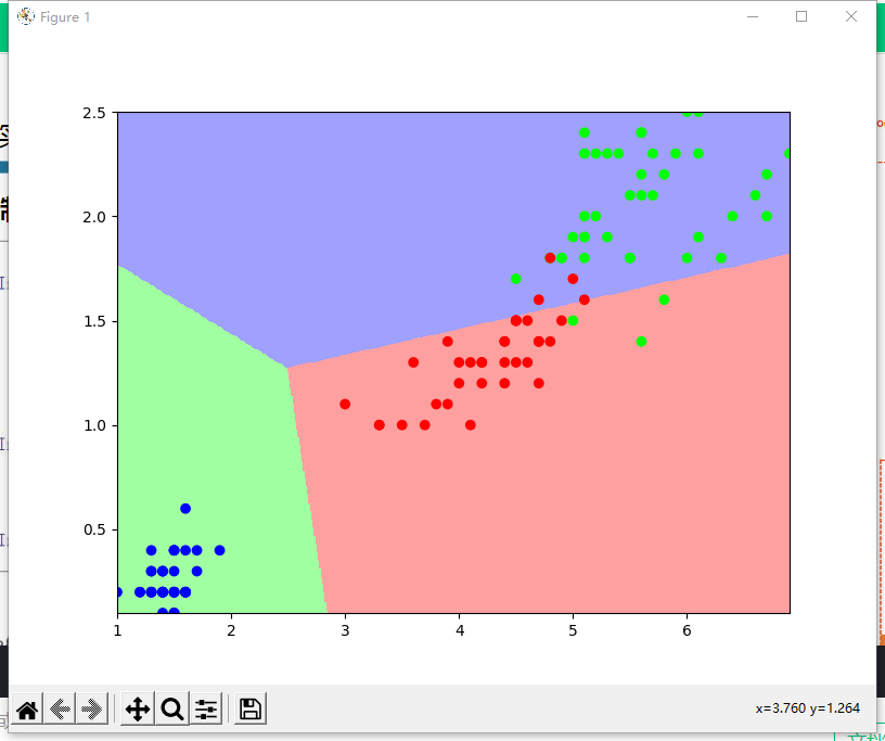
11.6.4.6 绘制分类图
M = 500
x1_min,x2_min = x_train.min(axis=0)
x1_max,x2_max = x_train.max(axis=0)
t1 = np.linspace(x1_min,x1_max,M)
t2 = np.linspace(x2_min,x2_max,M)
m1,m2 = np.meshgrid(t1,t2)

m0 = np.ones(M*M)
X_ = tf.cast(np.stack((m0,m1.reshape(-1),m2.reshape(-1)),axis=1),tf.float32)
Y_ = tf.nn.softmax(tf.matmul(X_,W))

Y_ = tf.argmax(Y_.numpy(),axis=1)

n = tf.reshape(Y_,m1.shape)

plt.figure(figsize = (8,6))
cm_bg =  mpl.colors.ListedColormap(['#A0FFA0','#FFA0A0','#A0A0FF'])

plt.pcolormesh(m1,m2,n,cmap=cm_bg)
plt.scatter(x_train[:,0],x_train[:,1],c = y_train,cmap="brg")

plt.show()
输出结果为:
11.6.4.7 本例代码汇总
import tensorflow as tf
import pandas as pd
import numpy as np
import matplotlib as mpl
import matplotlib.pyplot as plt

gpus = tf.config.experimental.list_physical_devices(device_type='GPU')
tf.config.experimental.set_memory_growth(gpus[0], True)

TRAIN_URL = "http://download.tensorflow.org/data/iris_training.csv"
TEST_URL = "http://download.tensorflow.org/data/iris_test.csv"

train_path = tf.keras.utils.get_file(TRAIN_URL.split('/')[-1],TRAIN_URL)
test_path = tf.keras.utils.get_file(TEST_URL.split('/')[-1],TEST_URL)

df_iris_train = pd.read_csv(train_path, header=0)

iris_train = np.array(df_iris_train)

x_train = iris_train[:,2:4]

y_train = iris_train[:,4]

num_train = len(x_train)

x0_train = np.ones(num_train).reshape(-1,1)
X_train = tf.cast(tf.concat([x0_train,x_train],axis=1),tf.float32)

Y_train = tf.one_hot(tf.constant(y_train,dtype=tf.int32),3)

learn_rate = 0.2
iter = 500
display_step = 100

np.random.seed(612)
W = tf.Variable(np.random.randn(3,3),dtype=tf.float32)

acc = []
cce = []

for i in range(0,iter+1):
    with tf.GradientTape() as tape:

        PRED_train = tf.nn.softmax(tf.matmul(X_train,W))

        Loss_train = -tf.reduce_sum(Y_train*tf.math.log(PRED_train))/num_train

    accuracy = tf.reduce_mean(tf.cast(tf.equal(tf.argmax(PRED_train.numpy(),axis=1),y_train),tf.float32))

    acc.append(accuracy)
    cce.append(Loss_train)

    dL_dW = tape.gradient(Loss_train,W)
    W.assign_sub(learn_rate*dL_dW)

    if i % display_step == 0:
        print("i: %i, Acc: %f, Loss: %f"%(i,accuracy,Loss_train))

print("自然顺序码为:" )
print(tf.argmax(PRED_train.numpy(),axis=1))

M = 500
x1_min,x2_min = x_train.min(axis=0)
x1_max,x2_max = x_train.max(axis=0)
t1 = np.linspace(x1_min,x1_max,M)
t2 = np.linspace(x2_min,x2_max,M)
m1,m2 = np.meshgrid(t1,t2)

m0 = np.ones(M*M)
X_ = tf.cast(np.stack((m0,m1.reshape(-1),m2.reshape(-1)),axis=1),tf.float32)
Y_ = tf.nn.softmax(tf.matmul(X_,W))

Y_ = tf.argmax(Y_.numpy(),axis=1)

n = tf.reshape(Y_,m1.shape)

plt.figure(figsize = (8,6))
cm_bg =  mpl.colors.ListedColormap(['#A0FFA0','#FFA0A0','#A0A0FF'])

plt.pcolormesh(m1,m2,n,cmap=cm_bg)
plt.scatter(x_train[:,0],x_train[:,1],c = y_train,cmap="brg")

plt.show()
11.7 参考文献
Original: https://blog.csdn.net/qq_45954434/article/details/121268688
Author: 踏破万里无云
Title: 【神经网络与深度学习-TensorFlow实践】-中国大学MOOC课程(十一)(分类问题))
原创文章受到原创版权保护。转载请注明出处:https://www.johngo689.com/665326/
转载文章受原作者版权保护。转载请注明原作者出处!