

实验二 数字图像的傅里叶变换
图像变换是数字图像处理中常用的技术,在图像增强、图像复原、图像压缩编码等数字图像处理中,都会用到图像变换技术,傅里叶变换是数字图像处理中应用最广的一种变换。
一、实验目的
(1)通过实验进一步加深对图像傅立叶变换的理解;
(2)计算离散图像的傅里叶变换;
(3)掌握图像的傅里叶频谱图及离散傅里叶变换性质;
(4)掌握 MATLAB 中的傅立叶变换函数;
(5)实现数字图像的傅立叶变换与反变换;
二、实验原理
对于数字图像 f(x,y),其二维离散傅立叶!

反变换公式为
图像的频率是表征图像中灰度变化剧烈程度的指标,是灰度在平面空间上的梯度。如:大面积的沙漠在图像中是一片灰度变化缓慢的区域,对应的频率值很低;而对于地表属性变换剧烈的边缘区域在图像中是一片灰度变化剧烈的区域,对应的频率值较高。傅里叶变换在实际中有非常明显的物理意义,设 f 是一 个能量有限的模拟信号,则其傅里叶变换就表示 f 的谱。从纯粹的数学意义上看,傅里叶变换是将一个函数转换为一系列周期函数来处理的。从物理效果看,傅里叶变换是将图像从空间域转换到频率域,其逆变换是将图像从频率域转换到空间域。换句话说,傅里叶变换的物理意义是将图像的灰度分布函数变换为图像的频率分布函数,傅里叶逆变换是将图像的频率分布函数变换为灰度分布函数。
另外说明以下几点:
- 图像经过二维傅里叶变换后,其变换系数矩阵表明:
若变换矩阵 Fn 原点设在中心,其频谱能量集中分布在变换系数矩阵的中心附近。若所用的二维傅里 叶变换矩阵 Fn 的原点设在左上角,那么图像信号能量将集中在系数矩阵的四个角上。这是由二维傅里叶 变换本身性质决定的。同时也表明一般图像能量集中低频区域。
2.变换之后的图像在原点平移之前四角是低频,最亮,平移之后中间部分是低频,最亮,亮度大说明
低频的能量大(幅角比较大)。
; 三、实验仪器及设备
计算机;MATLAB 图像处理软件;数字图像 lena.bmp,peppers.png 等
四、实验内容及步骤
- 查看 matlab 工具箱中二维傅立叶变换的相关函数;
二维傅里叶变换的 MATLAB 实现,是利用图像处理工具箱中的相关函数对给出的图像进行傅里叶变 换处理。在 MATLAB 中,相关函数如表 2.1 所示。
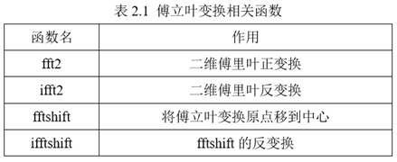
利用 help 命令查看相关函数用法。
help fft2
fft2 Two-dimensional discrete Fourier Transform.
fft2(X) returns the two-dimensional Fourier transform of matrix X.
If X is a vector, the result will have the same orientation.
fft2(X,MROWS,NCOLS) pads matrix X with zeros to size MROWS-by-NCOLS
before transforming.
help ifft2
ifft2 Two-dimensional inverse discrete Fourier transform.
ifft2(F) returns the two-dimensional inverse Fourier transform of matrix
F. If F is a vector, the result will have the same orientation.
ifft2(F,MROWS,NCOLS) pads matrix F with zeros to size MROWS-by-NCOLS
before transforming.
ifft2(…, ‘symmetric’) causes ifft2 to treat F as conjugate symmetric
in two dimensions so that the output is purely real. This option is
useful when F is not exactly conjugate symmetric merely because of
round-off error. See the reference page for the specific mathematical
definition of this symmetry.
ifft2(…, ‘nonsymmetric’) causes ifft2 to make no assumptions about the
symmetry of F.
help fftshift
fftshift Shift zero-frequency component to center of spectrum.
For vectors, fftshift(X) swaps the left and right halves of
X. For matrices, fftshift(X) swaps the first and third
quadrants and the second and fourth quadrants. For N-D
arrays, fftshift(X) swaps “half-spaces” of X along each
dimension.
fftshift(X,DIM) applies the fftshift operation along the
dimension DIM.
fftshift is useful for visualizing the Fourier transform with
the zero-frequency component in the middle of the spectrum.
help ifftshift
ifftshift Inverse FFT shift.
For vectors, ifftshift(X) swaps the left and right halves of
X. For matrices, ifftshift(X) swaps the first and third
quadrants and the second and fourth quadrants. For N-D
arrays, ifftshift(X) swaps “half-spaces” of X along each
dimension.
ifftshift(X,DIM) applies the ifftshift operation along the
dimension DIM.
ifftshift undoes the effects of FFTSHIFT.
- 熟练掌握 imread、imshow 函数。
利用 help 命令查看函数的用法。
help imread
imread Read image from graphics file.
A = imread(FILENAME,FMT) reads a grayscale or color image from the file
specified by the string FILENAME. FILENAME must be in the current
directory, in a directory on the MATLAB path, or include a full or
relative path to a file.
[X,MAP] = imread(FILENAME,FMT) reads the indexed image in FILENAME into
X and its associated colormap into MAP. Colormap values in the image
file are automatically rescaled into the range [0,1].
[…] = imread(FILENAME) attempts to infer the format of the file
from its content.
[…] = imread(URL,…) reads the image from an Internet URL.
help imshow
imshow Display image in Handle Graphics figure.
imshow(I) displays the grayscale image I.
imshow(I,[LOW HIGH]) displays the grayscale image I, specifying the display
range for I in [LOW HIGH]. The value LOW (and any value less than LOW)
displays as black, the value HIGH (and any value greater than HIGH) displays
as white. Values in between are displayed as intermediate shades of gray,
using the default number of gray levels.
imshow(I,[]) displays the grayscale image I scaling the display based
on the range of pixel values in I. imshow uses [min(I(😃) max(I(😃)] as
the display range, that is, the minimum value in I is displayed as
black, and the maximum value is displayed as white.
imshow(RGB) displays the truecolor image RGB.
imshow(BW) displays the binary image BW. imshow displays pixels with the
value 0 (zero) as black and pixels with the value 1 as white.
imshow(X,MAP) displays the indexed image X with the colormap MAP.
imshow(FILENAME) displays the image stored in the graphics file
FILENAME. The file must contain an image that IMREAD or DICOMREAD can
read. imshow calls IMREAD or DICOMREAD to read the image from the file,
but does not store the image data in the MATLAB workspace. If the file
contains multiple images, the first one will be displayed. The file
must be in the current directory or on the MATLAB path. (DICOMREAD
capability and the NITF file format require the Image Processing
Toolbox.)
- 利用 MATLAB 对图像进行离散傅里叶正变换及反变换,分析图像的傅里叶频谱。
图像一:一幅简单的数字图像
生成一幅大小为 512 _512 的黑色背景的中间叠加一个尺寸为 40_40 的白色矩阵的图像;
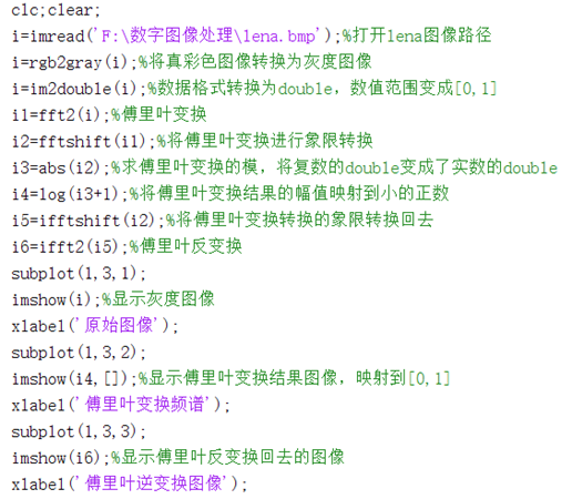
(1) 代码:
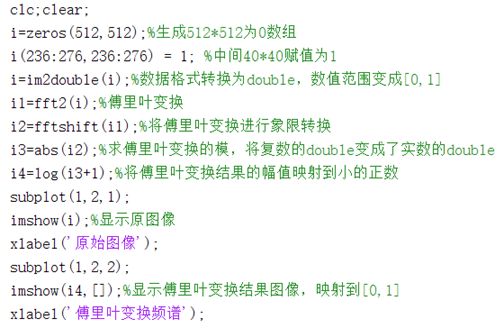
(2) 结果:
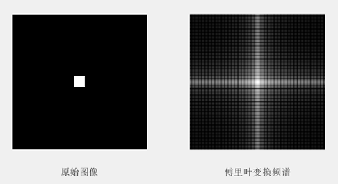
图一 傅里叶变换
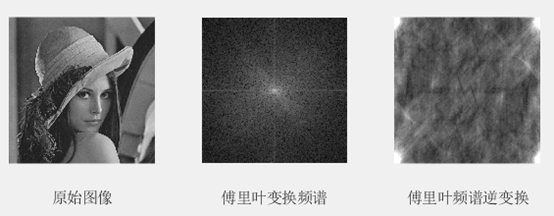
图像二:lena.bmp 或 peppers 图像
写出相应的数字图像的傅立叶反变换程序。
(1) 代码:
(2) 结果:
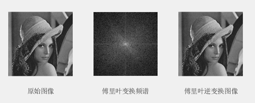
图二 傅里叶频谱
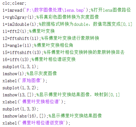
(3) 代码:
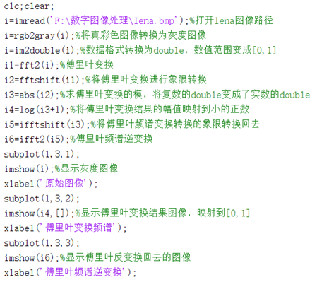
(4) 结果:
图三 傅里叶频谱
4 显示傅立叶变换的相位谱,并根据相位谱重建图像。分析由相位谱重建的图像。
(1) 代码:
(2)结果
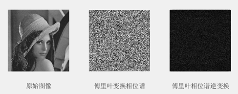
图四 傅里叶相位谱
图像的相位谱中,保留了图像的边缘以及整体结构的信息。
5 通过实验加深对傅立叶变换几个性质的理解,包括平移性质、尺度变换性质、旋转特性。
(1)平移性质:当空域中f(x,y)产生移动时,在频域中只发生相移,并不影响它的傅立叶变换的幅值。
代码:
clc;clear;
i1=zeros(512,512);%生成512*512为0数组
i1=im2double(i1);%数据格式转换为double,数值范围变成[0,1]
subplot(2,3,1);
i1(236:276,236:276) = 1; %中间40*40赋值为1
imshow(i1);
xlabel('原图像');
subplot(2,3,4);
i11=fft2(i1);%傅里叶变换
i12=fftshift(i11);%将傅里叶变换进行象限转换
i13=abs(i12);%求傅里叶变换的模,将复数的double变成了实数的double
i14=log(i13+1);%将傅里叶变换结果的幅值映射到小的正数
imshow(i14,[]);%显示傅里叶变换结果图像,映射到[0,1]
xlabel('原图像傅里叶谱');
subplot(2,3,2);
i2=zeros(512,512);
i2(236:276,384:424) = 1; %40*40赋值为1
imshow(i2);
xlabel('x轴平移图像');
subplot(2,3,5);
i21=fft2(i2);%傅里叶变换
i22=fftshift(i21);%将傅里叶变换进行象限转换
i23=abs(i22);%求傅里叶变换的模,将复数的double变成了实数的double
i24=log(i23+1);%将傅里叶变换结果的幅值映射到小的正数
imshow(i24,[]);%显示傅里叶变换结果图像,映射到[0,1]
xlabel('x轴平移傅里叶谱');
subplot(2,3,3);
i3=zeros(512,512);
i3(384:424,236:276) = 1; %40*40赋值为1
imshow(i3);
xlabel('y轴平移图像');
subplot(2,3,6);
i31=fft2(i3);%傅里叶变换
i32=fftshift(i31);%将傅里叶变换进行象限转换
i33=abs(i32);%求傅里叶变换的模,将复数的double变成了实数的double
i34=log(i33+1);%将傅里叶变换结果的幅值映射到小的正数
imshow(i34,[]);%显示傅里叶变换结果图像,映射到[0,1]
xlabel('y轴平移傅里叶谱');
结果:
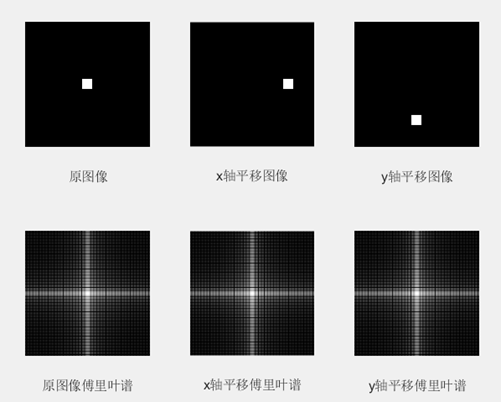
图五 傅里叶位移频谱变换规则
(2)尺度变换:当空域中f(x,y)产生缩放时,频域中傅立叶变换的幅值也相应的缩放。
代码:
clc;clear;
i=imread('F:\数字图像处理\lena.bmp');%打开lena图像路径
i=rgb2gray(i);%将真彩色图像转换为灰度图像
i1=im2double(i);%数据格式转换为double,数值范围变成[0,1]
i2=imresize(i1,0.2);%缩小
i3=imresize(i1,5);%放大

subplot(2,3,1);
imshow(i1);
xlabel('原图像');

subplot(2,3,4);
i11=fft2(i1);%傅里叶变换
i12=fftshift(i11);%将傅里叶变换进行象限转换
i13=abs(i12);%求傅里叶变换的模,将复数的double变成了实数的double
i14=log(i13+1);%将傅里叶变换结果的幅值映射到小的正数
imshow(i14,[]);%显示傅里叶变换结果图像,映射到[0,1]
xlabel('原图像傅里叶谱');

subplot(2,3,2);
imshow(i2);
xlabel('缩小图像');

subplot(2,3,5);
i21=fft2(i2);%傅里叶变换
i22=fftshift(i21);%将傅里叶变换进行象限转换
i23=abs(i22);%求傅里叶变换的模,将复数的double变成了实数的double
i24=log(i23+1);%将傅里叶变换结果的幅值映射到小的正数
imshow(i24,[]);%显示傅里叶变换结果图像,映射到[0,1]
xlabel('缩小图像傅里叶谱');

subplot(2,3,3);
imshow(i3);
xlabel('放大图像');
subplot(2,3,6);
i31=fft2(i3);%傅里叶变换
i32=fftshift(i31);%将傅里叶变换进行象限转换
i33=abs(i32);%求傅里叶变换的模,将复数的double变成了实数的double
i34=log(i33+1);%将傅里叶变换结果的幅值映射到小的正数
imshow(i34,[]);%显示傅里叶变换结果图像,映射到[0,1]
xlabel('放大图像傅里叶谱');
结果:
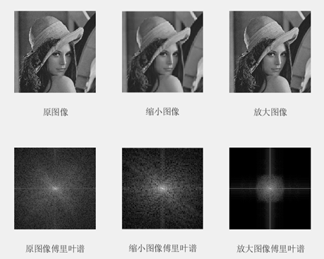
图六 放大缩小傅里叶频谱变换规则
(3)旋转特性:如果f(x,y)旋转了一个角度,那么对应的傅立叶变换也旋转了相同的角度。
代码:
clc;clear;
i=imread('F:\数字图像处理\lena.bmp');%打开lena图像路径
i=rgb2gray(i);%将真彩色图像转换为灰度图像
i1=im2double(i);%数据格式转换为double,数值范围变成[0,1]
i2=imrotate(i1,45);%旋转45°
i3=imrotate(i1,90);%旋转90°

subplot(2,3,1);
imshow(i1);
xlabel('原图像');

subplot(2,3,4);
i11=fft2(i1);%傅里叶变换
i12=fftshift(i11);%将傅里叶变换进行象限转换
i13=abs(i12);%求傅里叶变换的模,将复数的double变成了实数的double
i14=log(i13+1);%将傅里叶变换结果的幅值映射到小的正数
imshow(i14,[]);%显示傅里叶变换结果图像,映射到[0,1]
xlabel('原图像傅里叶谱');

subplot(2,3,2);
imshow(i2);
xlabel('旋转45°图像');

subplot(2,3,5);
i21=fft2(i2);%傅里叶变换
i22=fftshift(i21);%将傅里叶变换进行象限转换
i23=abs(i22);%求傅里叶变换的模,将复数的double变成了实数的double
i24=log(i23+1);%将傅里叶变换结果的幅值映射到小的正数
imshow(i24,[]);%显示傅里叶变换结果图像,映射到[0,1]
xlabel('旋转45°图像傅里叶谱');

subplot(2,3,3);
imshow(i3);
xlabel('旋转90°图像');
subplot(2,3,6);
i31=fft2(i3);%傅里叶变换
i32=fftshift(i31);%将傅里叶变换进行象限转换
i33=abs(i32);%求傅里叶变换的模,将复数的double变成了实数的double
i34=log(i33+1);%将傅里叶变换结果的幅值映射到小的正数
imshow(i34,[]);%显示傅里叶变换结果图像,映射到[0,1]
xlabel('旋转90°图像傅里叶谱');
结果:
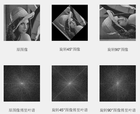
图七 图像旋转傅里叶频谱变换规则
五、实验心得
1.通过本次实验,我掌握了傅里叶变换与傅里叶逆变换的函数,知道如何求解傅里叶频谱与相位谱,并进行逆变换。
2.知道了空间域与频率域之间的区别与联系,以及在空间域中通过对图形进行相应的变换,它的频率域的变化规律。
3.不同的函数和求解方法,会产生不一样的傅里叶变换结果。
Original: https://blog.csdn.net/chengzilhc/article/details/118028498
Author: nochengzi
Title: 数字图像处理:实验二 数字图像的傅里叶变换
原创文章受到原创版权保护。转载请注明出处:https://www.johngo689.com/645017/
转载文章受原作者版权保护。转载请注明原作者出处!