【医学图像处理】用于肝血管分割的平均教师辅助置信学习

标题：Noisy Labels are Treasure: Mean-Teacher-Assisted Confident Learning for Hepatic Vessel Segmentation
作者：Donghuan Lu，腾讯天衍实验室；Xiu Li，清华大学深圳国际研究生院
来源：MICCAI 2021
代码：https://github.com/lemoshu/MTCL
主题：CT；图像分割；置信学习；迁移学习

1. 引言

❓ 论文想要解决的问题是什么？

由于肝血管的低对比度和复杂的形态学特征，从 CT 图像中手动分割肝血管比分割其他结构需要更多的专业知识和工作量，从而导致缺少高质量的肝血管标注数据，大多数数据都有相当多的未标记或标记错误的像素，也称为”噪声”。如果没有足够多的高质量标注数据，基于数据驱动的学习方法往往会遇到训练不足的问题。然而，输入低质量标注的数据可能会混淆网络，抵消高质量标注数据的有效性，导致性能下降。因此， 如何稳健地利用大量噪声标签数据中的附加信息仍然是一个挑战。

❓ 解决上述问题的现有方法有哪些？

为了充分利用低质量标注数据，一些减轻噪声标签带来的负面影响的方法如下：

• 对带有噪声标签的样本分配较小的权重 Zhu, Haidong, Jialin Shi, and Ji Wu. “Pick-and-learn: Automatic quality evaluation for noisy-labeled image segmentation.” International Conference on Medical Image Computing and Computer-Assisted Intervention. Springer, Cham, 2019.

• 对标签损坏的过程进行建模 Goldberger, Jacob, and Ehud Ben-Reuven. “Training deep neural-networks using a noise adaptation layer.” (2016).

• 置信学习 Northcutt, Curtis, Lu Jiang, and Isaac Chuang. “Confident learning: Estimating uncertainty in dataset labels.” Journal of Artificial Intelligence Research 70 (2021): 1373-1411.

2. 方法

2.1 数据集

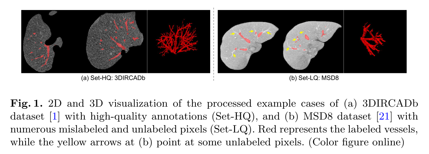
本研究使用两个公共数据集 3DIRCAb 和 MSD8，具有明显不同的注释质量，分别在本文中简称为 Set-HQ 和 Set-LQ。

1. 3DIRCADb：包含 20 张肝脏 CT 扫描图像，并提供高质量的肝脏和血管标注。
2. MSD8：包含 443 张肝脏 CT 扫描图像，但标注质量较低，大约 65.5% 的血管像素没有标记，大约 8.5% 的像素被错误地标记为血管。

在实验中，3DIRCADb 中的图像被随机分成两组：10 张用于训练，其余 10 张用于测试；MSD8 中的所有样本都只用于训练，因为它们的低质量噪声标签不适合用于评估。

; 2.2 数据处理

1. 裁剪图像：将所有图像裁剪到肝脏区域，图像大小为 320 × 320。
2. 归一化：将每个像素的亮度截断到 [−100, 250] HU 的范围，然后进行最小最大归一化。
3. 叠加概率图：我们观察到许多图像具有不同的强度范围和固有的图像噪声，这可能导致 模型对高强度区域过于敏感。因此，引入基于 Sato Tubeness 滤波器的血管概率图来提供辅助信息。通过计算 Hessian 矩阵的特征向量，可以获得图像与 tube 的相似性，从而增强潜在的血管区域。将血管概率图作为辅助图像，直接与经过处理的 CT 图像进行拼接。通过联合考虑图像和概率图中的信息，网络可以感知更稳健的血管信号以获得更好的分割性能。

2.3 MTCL 网络结构

本文提出的 Mean-Teacher-assisted Confident Learning (MTCL) 网络结构如下：

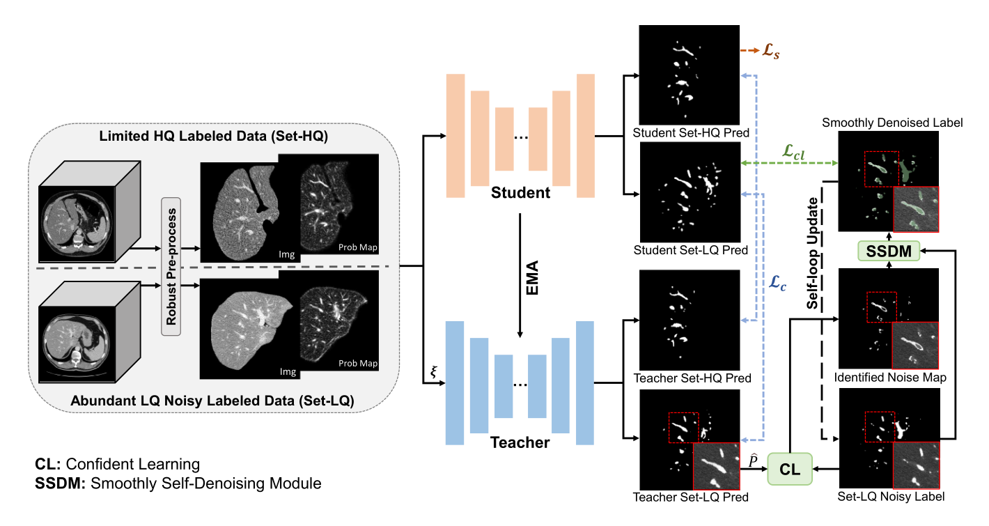
; 2.3.1 Mean Teacher Model

将训练步骤 t t t 中学生模型的权重表示为 θ t \theta_{t}θt ​， 指数移动平均（EMA） 用于更新教师模型的权重θ t ′ \theta_{t}^{\prime}θt ′​ ：θ t ′ = α θ t − 1 ′ + ( 1 − α ) θ t \theta_{t}^{\prime}=\alpha \theta_{t-1}^{\prime}+(1-\alpha) \theta_{t}θt ′​=αθt −1 ′​+(1 −α)θt ​ ，其中α \alpha α 是 EMA 衰减率并设置为 0.99 。通过最小化 Set-HQ 上的监督损失L s \mathcal{L}_{s}L s ​ 以及 两个数据集上学生模型和教师模型预测之间的无监督一致性损失 L c \mathcal{L}_{c}L c ​ 来优化学生模型。

2.3.2 Self-denoising Process

上述 Mean Teacher 模型只能利用图像信息，而噪声标签的潜在有用信息仍未被利用。为了在不受标签噪声影响的情况下进一步利用低质量标注，本文提出了一种渐进式自去噪过程。

置信学习

置信学习（Confident Learning, CL）的概念来自论文 Confident learning: Estimating uncertainty in dataset labels，用于找出的标注错误的样本。置信学习的主要过程如下图所示：

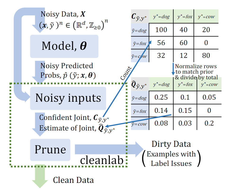
第一步：估计噪声标签y ~ \tilde{y}y ~​ 和真实标签y ∗ y^{*}y ∗ 的联合分布

给定具有 n n n 个样本和 m m m 个类别的数据集 X : = ( x , y ~ ) n \mathbf{X}:=(\mathbf{x}, \tilde{y})^{n}X :=(x ,y ~​)n，其中 y ~ \tilde{y}y ~​ 表示噪声标签（观察到的标签）。样本外预测概率 P ^ \hat{\boldsymbol{P}}P ^ 可以通过教师模型来获得。如果具有标签 y ~ = i \tilde{y}=i y ~​=i 的样本 x \mathbf{x}x 具有足够大的 p ^ j ( x ) ≥ t j \hat{p}{j}(\mathbf{x}) \geq t{j}p ^​j ​(x )≥t j ​，则可以怀疑 x \mathbf{x}x 的真实标签 y ∗ y^{*}y ∗ 是 j j j 而不是 i i i。这里，阈值 t j t_{j}t j ​ 是通过计算标签为 y ~ = j \tilde{y}=j y ~​=j 的样本的平均预测概率 p ^ j ( x ) \hat{p}_{j}(\mathbf{x})p ^​j ​(x ) 得到的：

t j : = 1 ∣ X y ~ = j ∣ ∑ x ∈ X y ~ = j p ^ j ( x ) t_{j}:=\frac{1}{\left|\mathbf{X}{\tilde{y}=j}\right|} \sum{\mathbf{x} \in \mathbf{X}{\tilde{y}=j}} \hat{p}{j}(\mathbf{x})t j ​:=∣X y ~​=j ​∣1 ​∑x ∈X y ~​=j ​​p ^​j ​(x )

在预测真实标签的基础上，进一步引入混淆矩阵 C y ~ , y ∗ \boldsymbol{C}_{\tilde{y}, y^{}}C y ~​,y ∗​，其中 C y ~ , y ∗ [ i ] [ j ] \mathbf{C}_{\tilde{y}, y^{}}[i][j]C y ~​,y ∗​[i ][j ] 是标签为 i i i、预测真实标签为 j j j 的 x \mathbf{x}x 的个数：

C y ~ , y ∗ [ i ] [ j ] : = ∣ X ^ y ~ = i , y ∗ = j ∣ \mathbf{C}{\tilde{y}, y^{}}[i][j]:=\left|\hat{\mathbf{X}}_{\tilde{y}=i, y^{}=j}\right|C y ~​,y ∗​[i ][j ]:=∣∣∣​X ^y ~​=i ,y ∗=j ​∣∣∣​，其中 X ^ y ~ = i , y ∗ = j : = { x ∈ X y ~ = i : p ^ j ( x ) ≥ t j , j = arg ⁡ max ⁡ l ∈ M : p ^ l ( x ) ≥ t l p ^ l ( x ) } \hat{\mathbf{X}}{\tilde{y}=i, y^{*}=j}:=\left{\mathbf{x} \in \mathbf{X}{\tilde{y}=i}: \hat{p}{j}(\mathbf{x}) \geq t_{j}, j=\underset{l \in M: \hat{p}{l}(\mathbf{x}) \geq t{l}}{\arg \max } \hat{p}_{l}(\mathbf{x})\right}X ^y ~​=i ,y ∗=j ​:={x ∈X y ~​=i ​:p ^​j ​(x )≥t j ​,j =l ∈M :p ^​l ​(x )≥t l ​ar g max ​p ^​l ​(x )}

利用构造的混淆矩阵 C y ~ , y ∗ \boldsymbol{C}_{\tilde{y}, y^{}}C y ~​,y ∗​，我们可以进一步得到 m × m m \times m m ×m 联合分布矩阵 Q y ~ , y ∗ \mathbf{Q}_{\tilde{y}, y^{}}Q y ~​,y ∗​：

Q y ~ , y ∗ [ i ] [ j ] = C y ~ , y ∗ [ i ] [ j ] ∑ j ∈ M C y ~ , y ∗ [ i ] [ j ] ⋅ ∣ X y ~ = i ∣ ∑ i ∈ M , j ∈ M ( C y ~ , y ∗ [ i ] [ j ] ∑ j ∈ M C y ~ , y ∗ [ i ] [ j ] ⋅ ∣ X y ~ = i ∣ ) \mathbf{Q}{\tilde{y}, y^{}}[i][j]=\frac{\frac{\mathbf{C}_{\tilde{y}, y^{}}[i][j]}{\sum{j \in M} \mathbf{C}{\tilde{y}, y^{}}[i][j]} \cdot\left|\mathbf{X}{\tilde{y}=i}\right|}{\sum{i \in M, j \in M}\left(\frac{\mathbf{C}_{\tilde{y}, y^{}}[i][j]}{\sum{j \in M} \mathbf{C}{\tilde{y}, y^{*}}[i][j]} \cdot\left|\mathbf{X}{\tilde{y}=i}\right|\right)}Q y ~​,y ∗​[i ][j ]=∑i ∈M ,j ∈M ​(∑j ∈M ​C y ~​,y ∗​[i ][j ]C y ~​,y ∗​[i ][j ]​⋅∣X y ~​=i ​∣)∑j ∈M ​C y ~​,y ∗​[i ][j ]C y ~​,y ∗​[i ][j ]​⋅∣X y ~​=i ​∣​

第二步：找出错误标记的样本

本文利用论文 Confident learning: Estimating uncertainty in dataset labels 中介绍的 Prune by Class (PBC) 方法识别标签噪声。具体地说，对于每个类别 i i i，PBC 选择 n ⋅ ∑ j ∈ 1 , 2 , … m : j ≠ i Q y ~ , y ∗ [ i ] [ j ] n \cdot \sum_{j \in 1,2, \ldots m: j \neq i} \mathbf{Q}{\tilde{y}, y^{*}}[i][j]n ⋅∑j ∈1 ,2 ,…m :j ​=i ​Q y ~​,y ∗​[i ][j ] 个具有最低置信度 p ^ ( y ~ = i ; x ∈ X i ) \hat{p}\left(\tilde{y}=i ; \boldsymbol{x} \in \boldsymbol{X}{i}\right)p ^​(y ~​=i ;x ∈X i ​) 的样本作为错误标记的样本，从而得到二值噪声识别图（binary noise identification map）X n \mathbf{X}_{n}X n ​，其中”1″表示像素具有错误的标记。

关于置信学习更详细的知识可以参考以下资料：

1. Northcutt, Curtis, Lu Jiang, and Isaac Chuang. “Confident learning: Estimating uncertainty in dataset labels.” Journal of Artificial Intelligence Research 70 (2021): 1373-1411.

2. 置信学习-标注数据存在错误 – 知乎 (zhihu.com)

; 标签平滑

置信学习在识别标签噪声方面仍然存在不确定性。因此，本研究中没有直接进行硬校正，而是引入了平滑自去噪模块（Smoothly Self-Denoising Module, SSDM）来对给定的噪声分割掩模 y ~ \tilde{y}y ~​ 进行软校正。基于二值噪声识别图 X n \mathbf{X}_{n}X n ​，平滑自去噪操作可以表示为：

y ˙ ( x ) = y ~ ( x ) + I ( x ∈ X n ) ⋅ ( − 1 ) y ~ ⋅ τ \dot{y}(\mathbf{x})=\tilde{y}(\mathbf{x})+\mathbb{I}\left(\mathbf{x} \in \mathbf{X}_{n}\right) \cdot(-1)^{\tilde{y}} \cdot \tau y ˙​(x )=y ~​(x )+I (x ∈X n ​)⋅(−1 )y ~​⋅τ

其中 I ( ⋅ ) \mathbb{I}(\cdot)I (⋅) 为指示函数，τ ∈ [ 0 , 1 ] \tau \in[0,1]τ∈[0 ,1 ] 为平滑因子，根据经验设置为 0.8。

2.4 损失函数

总损失是 Set-HQ 上的监督损失 L s \mathcal{L}{s}L s ​、两个数据集上的扰动一致性损失 L c \mathcal{L}{c}L c ​ 和 Set-LQ 上的辅助自去噪置信学习损失 L c l \mathcal{L}_{c l}L c l ​ 的加权组合，计算公式为：

L = L s + λ c L c + λ c l L c l \mathcal{L}=\mathcal{L}{s}+\lambda{c} \mathcal{L}{c}+\lambda{c l} \mathcal{L}_{c l}L =L s ​+λc ​L c ​+λc l ​L c l ​

其中 λ c \lambda_{c}λc ​ 和 λ c l \lambda_{c l}λc l ​ 分别是 L c \mathcal{L}{c}L c ​ 和 L c l \mathcal{L}{c l}L c l ​ 的权重。

在不同的步骤中使用不同的 λ c \lambda_{c}λc ​，根据论文 Semi-supervised Brain Lesion Segmentation with an Adapted Mean Teacher Model，λ c = exp ⁡ ( − 5 ( 1 − S L ) 2 ) ( when S ≤ L ) \lambda_{c}=\exp \left(-5\left(1-\frac{S}{L}\right)^{2}\right)(\text { when } S \leq L)λc ​=exp (−5 (1 −L S ​)2 )(when S ≤L )，其中 S S S 是当前的训练步数，L L L 称为斜升长度，根据经验设置 L = 400 L =400 L =4 0 0。当 S > L S > L S >L 时，λ c \lambda_{c}λc ​ 设置为 1。同时，教师模型需要”预热”以提供可靠的样本外预测概率。因此，λ c l \lambda_{c l}λc l ​ 在前 4000 次迭代中设置为 0，在其余训练迭代中调整为 0.5。

监督损失 L s \mathcal{L}{s}L s ​ 是交叉熵损失、Dice 损失、 焦点损失（Focal Loss）和 边界损失（Boundary Loss）的组合，权重分别为 0.5、0.5、1 和 0.5。一致性损失 L c \mathcal{L}{c}L c ​ 由体素均方误差 (MSE) 计算得出，而置信学习损失 L c l \mathcal{L}_{c l}L c l ​ 由等权重的交叉熵损失和焦点损失组成。

3. 实验过程与结果

3.1 实施

• 硬件： NVIDIA Titan X GPU
• 框架：PyTorch
• 数据增强：随机翻转和旋转
• 优化器：SGD
• 批量大小：4
• 评估指标：Dice 得分、精度（PRE）、平均表面距离（Average Surface Distance, ASD）和 Hausdorff 距离（HD）

3.2 对比研究和消融研究

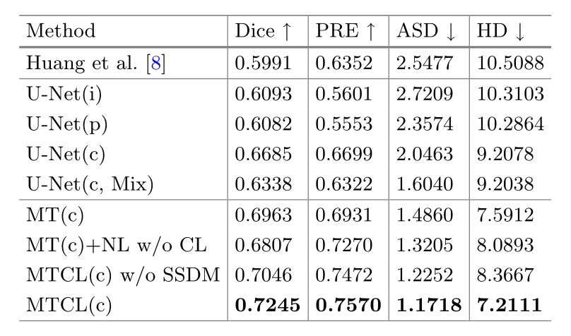
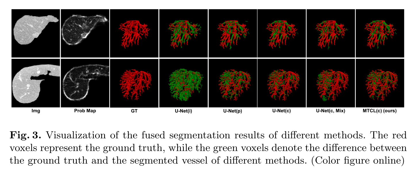
对 Set-HQ 的测试集进行了比较研究，实验结果如下表和下图所示。”i”、”p”和”c”代表不同的输入类型：预处理后的图像、血管概率图以及两者拼接后的图像。可以发现，本文所提出的方法（表示为 MTCL©）在所有四个指标和视觉结果上都具有最佳性能。

U-Net(c, Mix) 表示在训练中使用了 Set-LQ。正如预测的那样，实验结果表明 Set-LQ 的噪声标签会导致不可避免的性能下降。

为了验证每个组件的有效性，我们使用以下变体进行了消融研究：（1） MT©：典型的 mean-teacher 模型（2） MT©+NL w/o CL：在 MT©的基础上，额外使用用 Set-LQ 的噪声标签（noisy labels, NL），没有 CL；（3） MTCL© w/o SSDM：没有 SSDM 的 MTCL。如表中结果所示，在 Set-LQ 的图像信息的辅助下，加入扰动一致性损失可以提高分割性能，同时缓解噪声标签导致的性能下降。通过 CL 的自去噪过程可以实现卓越的性能，并通过 SSDM 进一步改进。

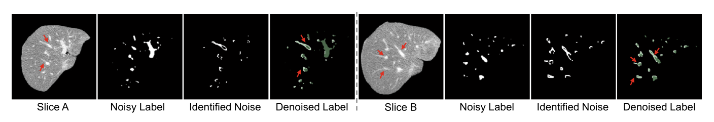
; 3.3 验证标签自去噪的有效性

来自 MSD8 的两个示例切片的可视化如下图所示，以进一步说明标签自去噪过程。结果表明，本文提出的网络可以识别出一些明显的噪声，提高噪声标记数据的质量。

4. 重要参考文献

• Mean-teacher Model Tarvainen, Antti, and Harri Valpola. “Mean teachers are better role models: Weight-averaged consistency targets improve semi-supervised deep learning results.” arXiv preprint arXiv:1703.01780 (2017). Cui, Wenhui, et al. “Semi-supervised brain lesion segmentation with an adapted mean teacher model.” International Conference on Information Processing in Medical Imaging . Springer, Cham, 2019.

• 置信学习 Confident Learning Northcutt, Curtis, Lu Jiang, and Isaac Chuang. “Confident learning: Estimating uncertainty in dataset labels.” Journal of Artificial Intelligence Research 70 (2021): 1373-1411. Zhang, Minqing, et al. “Characterizing label errors: Confident learning for noisy-labeled image segmentation.” International Conference on Medical Image Computing and Computer-Assisted Intervention . Springer, Cham, 2020.

• 标签平滑 Label Smoothing Ainam, Jean-Paul, et al. “Sparse label smoothing regularization for person re-identification.” IEEE Access 7 (2019): 27899-27910.

• 焦点损失 Focal Loss Lin, Tsung-Yi, et al. “Focal loss for dense object detection.” Proceedings of the IEEE international conference on computer vision . 2017.

• 边界损失 Boundary Loss Kervadec, Hoel, et al. “Boundary loss for highly unbalanced segmentation.” International conference on medical imaging with deep learning . PMLR, 2019.

5. 评审意见

官方评审意见 👉https://miccai2021.org/openaccess/paperlinks/2021/09/01/343-Paper0008.html

5.1 优点

• Datasets with bad segmentation quality are still quite common, so this method addresses an important problem which can be helpful to the community.

• Nice set of contributions including vessel probability map use (from Sato tubeless filter) as auxiliary input modality and adaptation of confident learning in a mean-teacher learning segmentation framework.

• Methodological contributions are assessed rigorously through a detailed ablation study.

5.2 缺点

• The authors applied their method to only the single problem of hepatic vessel segmentation, and all empirical results are derived from a test set with only ten segmented cases. Because of this, even though the results look promising, it’s difficult to be sure that this is not just a lucky coincidence. No attempt is made to demonstrate the statistical significance of the reported improvement.

• Lack of comparisons with respect to state-of-the-art (Huang et al. and standard U-Net only).

5.3 建议

• I feel that this paper would be far stronger if the same experiments had been conducted on one or two other similar problems – perhaps ones in which HQ test sets with more than ten cases are possible. Here, you will have far more statistical power to demonstrate that your results are not just a statistical anomaly.

• The high-quality annotated dataset is randomly divided into two groups (10 cases for training, 10 for test). The article does not mention any cross-validation strategy. Do you use cross-validation to strengthen the effectiveness of the obtained results? Even if the 3DIRCADb dataset is relatively small, you should include a validation subset to find the optimal network hyper-parameters.

• I would suggest you to use other state-of-the-art methods additionally to Huang et al. and standard U-Net to improve the experimental part.

• It is a bit startling to still see papers without any statistical test. Performance gains could be confirmed using t-tests.

• Reporting average numbers are not enough – we need more information on the error distribution (min/max/std). Actually in this case, since there are only 10 validation cases, it would have been possible to report the numbers for each case individually.

• I am not sure if the experiment comparing training on the HQ+LQ data vs training only on HQ data is fair. Since there are much more LQ data, it seems that training on HQ+LQ means training on LQ only. The HQ should be sampled much more often so that an HQ image appears as often as a LQ one.

• The decision to not resample in the z-direction is very surprising. If the slice thickness changes, the network has to unnecessarily learn structures with a different size in this direction. I do not understand the invoked rationale of “avoiding resampling artifacts”. Furthermore this is even acknowledged by the authors when they report that 3D networks are worse than 2D ones.

Original: https://blog.csdn.net/weixin_61033221/article/details/122743169
Author: 菜鸟刘同学
Title: 【医学图像处理】用于肝血管分割的平均教师辅助置信学习