

GSVA 也是 SCI 文章中常见的分析方法,在我们获得多个pathway的时候,可以比较pathway在样本分组中的差异,这样可以更好的确定每个通络的活性。
前言
GSVA全名Gene set variation analysis(基因集变异分析),是一种非参数,无监督的算法。与GSEA不同,GSVA不需要预先对样本进行分组,可以计算每个样本中特定基因集的富集分数。换而言之,GSVA转化了基因表达数据,从单个基因作为特征的表达矩阵,转化为特定基因集作为特征的表达矩阵。GSVA对基因富集结果进行了量化,可以更方便地进行后续统计分析。如果用limma包做差异表达分析可以寻找样本间差异表达的基因,同样地,使用limma包对GSVA的结果(依然是一个矩阵)做同样的分析,则可以寻找样本间有显著差异的基因集。这些”差异表达”的基因集,相对于基因而言,更加具有生物学意义,更具有可解释性,可以进一步用于肿瘤subtype的分型等等与生物学意义结合密切的探究。
文章中摘要
背景:基因集富集(GSE)分析是一种流行的基因信息浓缩框架将配置文件表达为路径或签名摘要。 这种方法比单基因分析的优势包括降低噪音和尺寸,以及更大的生物可解释性。分子分析实验超越了简单的病例对照研究,需要强有力和灵活的GSVA方法在高度异构的数据集中建模路径活动。
结果:为了解决这一挑战,我们引入了基因集变异分析(GVSA),一个GVSA方法估计以无监督的方式在样本群体上的途径活性变化。我们证明了GVSA与当前最先进的取样富集方法的比较。 此外,我们提供的例子它在差异通路活性和生存分析中的应用。最后,我们将展示GVSA如何以类似的方式处理数据从微阵列和RNA测序实验。
结论:GVSA提供了更强的能力来检测在样本人群中微妙的通路活性变化相应方法的比较,而GSE方法通常被认为是生物信息学的终点分析表明,GVSA是构建生物通路中心模型的起点。 此外,GVSA有助于当前对RNA-seq数据的GVSA方法的需求。


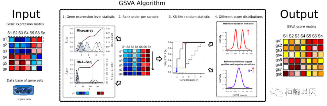
GSVA方法的基本原理 GSA是一个以log2微阵列表达值或RNA-seq计数形式的基因表达矩阵和一个基因集数据库。
- 累积密度函数(KCDF)的核估计。这两个图显示了两个模拟表达谱,模拟了来自微阵列和RNA-seq数据的6个样本。x轴对应的是4个样本中每个基因表达量较低,另外2个样本中表达量较高的表达量。KCDF尺度在左y轴,高斯核和泊松核的尺度在右y轴;
- 表达式级统计量对每个样本进行排序;3.对每个基因集,计算类kolmogorov -smirnov秩统计量。图中显示了一个由10个基因中的3个组成的基因集,并对基因集内外的基因进行了抽样计算;
- GSA浓缩分数要么是对零的最大偏差(上),要么是两个和的差值(下)。这两个图显示了在基因表达无变化的零假设下的两种模拟结果得分(见正文)。该算法的输出是一个矩阵,包含每个基因集和样本的路径富集分数。
; 实例解析
1.软件安装
软件包就是 GSVA ,安装并加载,后面的函数基本来自于这个包,如下:
if (!require("BiocManager", quietly = TRUE)) {
    install.packages("BiocManager")
}
if (!require("GSVA", quietly = TRUE)) {
    BiocManager::install("GSVA")
}
if (!require("GSEABase", quietly = TRUE)) {
    BiocManager::install("GSEABase")
}
if (!require(clusterProfiler)) {
    BiocManager::install("clusterProfiler")
}
library(GSVA)
library(GSEABase)
library(clusterProfiler)
2.数据读取
数据要求
1、特定感兴趣的基因集(如信号通路,GO条目等),列出基因集中基因
2、基因表达矩阵,为经过log2标准化的芯片数据或者RNA-seq count数数据(基因名形式与基因集对应)
我们仍然使用的是 TCGA-COAD的数据集,表达数据的读取以及临床信息分组的获得我们上期已经提过,我们使用的是edgeR 软件包计算出来的差异表达结果,提取上调基因 2832 的 ENSEMBL号如下:
DEG = read.table("DEG-resdata.xls", sep = "\t", check.names = F, header = T)
group <- 1296 2832 read.table("deg-group.xls", sep="\t" , check.names="F," header="T)" table(deg$sig) ## down up exp <- deg[, c(1, 8:ncol(deg))] < code></->
3.替换基因名称
在做GSVA分析时我们需要将基因编码统一为”ENSEMBL”,才可以注释成功,所以我们需要利用软件包clusterProfiler转下基因编码,如下:
eg <- 1 2 3 4 5 6 7123 8029 130749 200931 266675 284723 bitr(exp$row.names, fromtype="ENSEMBL" , totype="c("ENTREZID"," "ensembl", "symbol"), orgdb="org.Hs.eg.db" ) ## warning in : 30.89% of input gene ids are fail to map... head(eg) ensembl entrezid symbol ensg00000142959 best4 ensg00000163815 clec3b ensg00000107611 cubn ensg00000162461 slc25a34 ensg00000163959 slc51a ensg00000144410 cpo mergedata <- merge(eg, exp, by.x="ENSEMBL" by.y="Row.names" mergedata[!duplicated(mergedata$symbol), ] expmatrix mergedata[, 4:ncol(mergedata)] rownames(expmatrix)="mergedata[," 2] < code></->
3.GSVA分析
需要gmt文件,http://www.gsea-msigdb.org/gsea/downloads.jsp 路径下载,选择合适的,我们这里是结直肠癌中癌和癌旁的差异比较分析,所以我们需要找到致癌基因,选择 c5: Ontology gene sets 即 c5.all.v7.5.1.entrez.gmt 文件,然后进行 GSVA 富集分析,因为我们的数据是 Read Count,因此我们在算法上选择”Poission”, 如下:
geneSets <- 4 519 8966 getgmt('c5.all.v7.5.1.entrez.gmt') ###下载的基因集 gsva_hall <- gsva(expr="as.matrix(expMatrix)," gset.idx.list="geneSets," # method="gsva" , #c("gsva", "ssgsea", "zscore", "plage") mx.diff="T," 数据为正态分布则t,双峰则f kcdf="Poisson" #cpm, rpkm, tpm数据就用默认值"gaussian", read count数据则为"poisson", parallel.sz="4,#" 并行线程数目 min.sz="2)" ## warning in multicoreparam(progressbar="verbose," workers="parallel.sz," : multicoreparam() not supported on windows, use snowparam() setting parallel calculations through a multicoreparam back-end with and tasks="100." estimating gsva scores for gene sets. ecdfs poisson kernels cores gsva_hall[1:5,1:3] tcga-3l-aa1b-01a-11r-a37k-07 gobp_reproduction 0.03836725 gobp_regulation_of_dna_recombination -0.75104749 gobp_very_long_chain_fatty_acid_metabolic_process 0.55088900 gobp_transition_metal_ion_transport 0.06202858 gobp_mitotic_sister_chromatid_segregation -0.52998248 tcga-4n-a93t-01a-11r-a37k-07 -0.124108558 -0.001155191 0.414166085 -0.262603823 -0.123013569 tcga-4t-aa8h-01a-11r-a41b-07 -0.1063165 -0.4464710 -0.2267969 -0.1875599 -0.1757369 dim(gsva_hall) [1] < code></->
4.limma差异通路分析
由于我们获得的结果很多,所以随机抽取一些做后续分析,如下:
library(limma)
设置或导入分组
table(group$Group)
##
##  NT  TP
##  41 478
design <- 0 1 model.matrix(~0 + group$group) colnames(design)="levels(factor(group$Group))" rownames(design)="colnames(GSVA_hall)" head(design) ## nt tp tcga-3l-aa1b-01a-11r-a37k-07 tcga-4n-a93t-01a-11r-a37k-07 tcga-4t-aa8h-01a-11r-a41b-07 tcga-5m-aat4-01a-11r-a41b-07 tcga-5m-aat5-01a-21r-a41b-07 tcga-5m-aat6-01a-11r-a41b-07 # tumor vs normal compare <- makecontrasts(tp - nt, levels="design)" fit lmfit(gsva_hall, design) fit2 contrasts.fit(fit, compare) fit3 ebayes(fit2) diff toptable(fit3, coef="1," number="8966)" head(diff) logfc aveexpr gomf_guanyl_nucleotide_binding -0.7011267 -0.10083405 gobp_cellular_carbohydrate_metabolic_process -0.5638841 -0.07316197 gobp_organophosphate_biosynthetic_process -0.5945028 -0.07437185 gobp_cellular_response_to_steroid_hormone_stimulus -0.6657586 -0.10911896 gobp_organophosphate_metabolic_process -0.4911074 -0.07047891 gobp_intracellular_receptor_signaling_pathway -0.5988359 -0.07267329 t p.value -17.70510 2.666079e-55 -17.41117 6.923672e-54 -17.26777 3.374256e-53 -17.01655 5.363531e-52 -16.59499 5.420659e-50 -16.29934 1.351446e-48 adj.p.val b 2.390406e-51 115.00527 3.103882e-50 111.77783 1.008453e-49 110.20837 1.202235e-48 107.46743 9.720326e-47 102.89368 2.019512e-45 99.70696 < code></->
结果展示
结果展示又有多种方式,可以对整体绘制热图,也可以绘制条形图,又或者细致分析一下每个pathway和对应基因的生存情况等等。
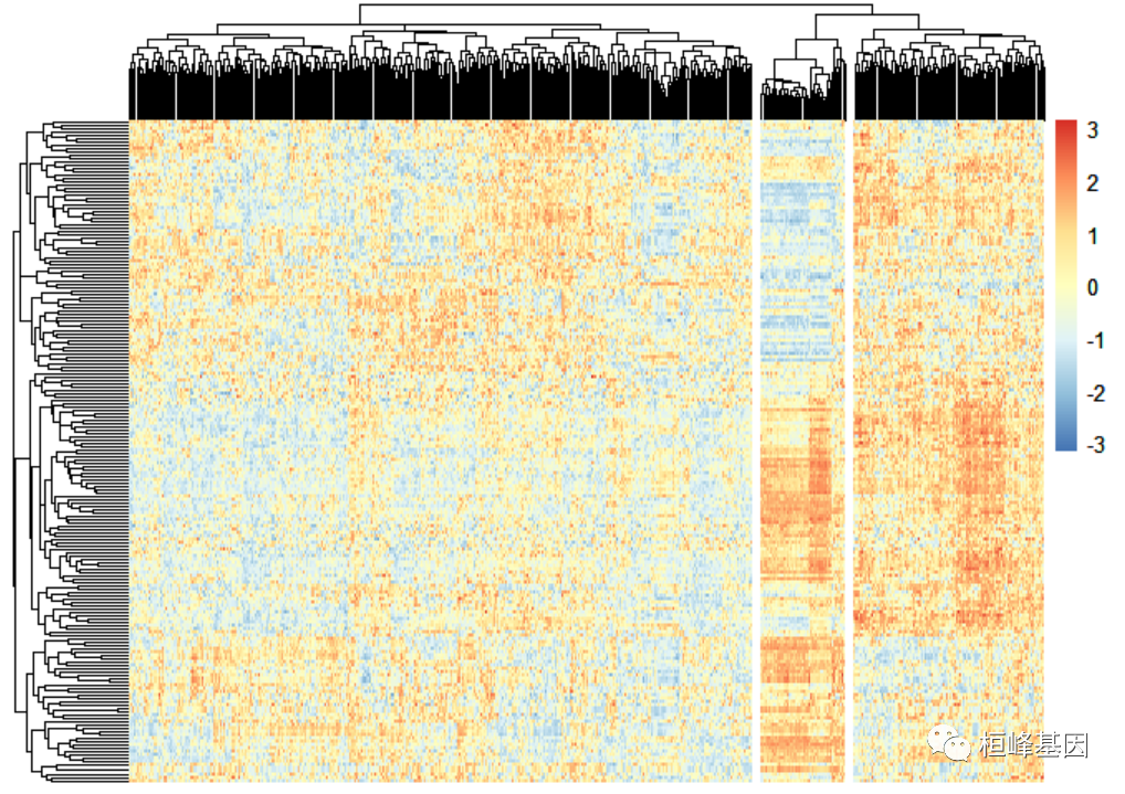
1.绘制热图
根据分值,还画了一个热图,以此为依据进行无监督分类,看通路活动相似的样本是否有特殊的生物含义。
随机抽取200个
library(dplyr)
set.seed(1234)
GSVA_Sample <- 200 519 sample_n(as.data.frame(gsva_hall), 200, replace="FALSE)" gsvamatrix <- t(scale(t(gsva_sample))) # 标准h normalization function(x) { return((x - min(x)) (max(x) min(x))) } norgsvamatrix normalization(gsvamatrix) dim(norgsvamatrix) ## [1] score.gsva.metab="as.data.frame(t(norgsvaMatrix))" score.gsva.metab[1:5, 1:3] hp_redundant_neck_skin hp_sensory_ataxia tcga-3l-aa1b-01a-11r-a37k-07 0.4414314 0.6195093 tcga-4n-a93t-01a-11r-a37k-07 0.3025181 0.7938041 tcga-4t-aa8h-01a-11r-a41b-07 0.6276248 0.6352028 tcga-5m-aat4-01a-11r-a41b-07 0.2068621 0.7342094 tcga-5m-aat5-01a-21r-a41b-07 0.3116117 0.6989451 hp_progressive 0.7002951 0.5197090 0.4727434 0.4766886 0.5829184 library(pheatmap) p pheatmap(norgsvamatrix, scale="row" , show_colnames="F," show_rownames="F," cluster_cols="T," cluster_rows="T," cex="1," clustering_distance_rows="euclidean" clustering_distance_cols="euclidean" clustering_method="complete" border_color="FALSE," cutree_col="3)" < code></->
cluster = cutree(p$tree_col, k = 3)  #from left to right 1 3 2
table(cluster)
## cluster
##   1   2   3
## 110 360  49
2.绘制发散条形图
最后就是展示结果这部分来自网络高手的绘图代码,也是文章中出现的模式,如下:
## barplot
set.seed(1234)
Diff_sample<-sample_n(diff, 30, replace="FALSE)" dat_plot <- data.frame(id="row.names(Diff_sample)," t="Diff_sample$t)" # 去掉"hallmark_" library(stringr) dat_plot$id str_replace(dat_plot$id , "hallmark_","") 新增一列 根据t阈值分类 dat_plot$threshold="factor(ifelse(dat_plot$t">-2, ifelse(dat_plot$t >= 2 ,'Up','Stable'),'Down'),levels=c('Up','Down','Stable'))
排序
dat_plot <- dat_plot %>% arrange(t)
变成因子类型
dat_plot$id <- factor(dat_plot$id,levels="dat_plot$id)" # 绘制 library(ggplot2) library(ggthemes) ## warning: 程辑包'ggthemes'是用r版本4.1.3 来建造的 install.packages("ggprism") library(ggprism) 程辑包'ggprism'是用r版本4.1.3 p <- ggplot(data="dat_plot,aes(x" = id,y="t,fill" threshold)) + geom_col()+ coord_flip() scale_fill_manual(values="c('Up'=" '#36638a','nosignifi'="#cccccc" ,'down'="#7bcd7b" )) geom_hline(yintercept="c(-2,2)," color="white" , size="0.5," lty="dashed" ) xlab('') ylab('t value of gsva score, tp-vs-nt') #注意坐标轴旋转了 guides(fill="F)+" 不显示图例 theme_prism(border="T)" theme( axis.text.y="element_blank()," axis.ticks.y="element_blank()" guides(<scale> = FALSE) is deprecated. Please use guides(<scale> =
## "none") instead.
添加标签
此处参考了:https://mp.weixin.qq.com/s/eCMwWCnjTyQvNX2wNaDYXg
小于-2的数量
low1 <- dat_plot %>% filter(t < -2) %>% nrow()
小于0总数量
low0 <- dat_plot %>% filter( t < 0) %>% nrow()
小于2总数量
high0 <- dat_plot %>% filter(t < 2) %>% nrow()
总的柱子数量
high1 <- nrow(dat_plot) # 依次从下到上添加标签 p + geom_text(data="dat_plot[1:low1,],aes(x" = id,y="0.1,label" id), hjust="0,color" 'black',size="2.5)" 小于-1的为黑色标签 +1):low0,],aes(x="id,y" 0.1,label="id)," 'grey',size="2.5)" 灰色标签 1):high0,],aes(x="id,y" -0.1,label="id)," +1):high1,],aes(x="id,y" 大于1的为黑色标签 < code></-></-></-></-></scale></-></-></-sample_n(diff,>

#ggsave("gsva_bar.pdf",p,width = 15,height = 15)
结果解读
计算GSVA 分值,按rank从大到小排序作为X轴,按照基因集内(红线)和基因集外(绿线)画两条K-S 统计分布线,遇见符合要求(集内/集外)的基因”升级”,越前则”升级”幅度越大,与表达量成正比。(In other words we are rising proportional to how much a gene is expressed)。 求”基因集内基因分布”和”基因集外基因分布”两者之间的最大偏差。两者之间的偏差可以是正方向和负方向,它们的差值作为 GSVA 分值。

GSVA 分数含义
- 当S1分值 = 0.57,基因集内基因的表达多于基因集外基因,通路活性上调;
- 当S2分值 = -0.71, 基因集内基因表达低于基因集外基因,通路活性下降;
- 当S3分值 = 0.1, 接近零,说明基因集内外基因表达模式差别不大。
; 文献解读
现在我们看下文章中是怎么利用GSVA来做分析,选取文章如下:
在文章中作为主体单独出现的一部分,详细描述了该方法使用的过程,如下:
Identification of pathways that are differentially expressed with increasing disease activity and fibrosis stage We next used the Gene Set Variation Analysis (GSVA) which allows the ordinal histological severity score to be regressed against pathway-level abundance values. Whereas the PPI network analysis enabled the discovery of communities of genes that are coordinately regulated, the GSVA analysis allowed us to identify specific, established pathways that are differentially regulated with increasing histological severity. Using both approaches allowed us to identify both the biological pathways perturbed across increasing disease severity as well as the relationship between the processes that are perturbed.
我们看下结果获得每个Pathway的差异分析结果,如下:

并且挑选重点的pathway进一步分析其Score值,并作图如下:

References:
-
Hoang, S.A., Oseini, A., Feaver, R.E. et al. Gene Expression Predicts Histological Severity and Reveals Distinct Molecular Profiles of Nonalcoholic Fatty Liver Disease. Sci Rep 9, 12541 (2019).
-
Hänzelmann S, Castelo R, Guinney J. GSVA: gene set variation analysis for microarray and RNA-seq data. BMC Bioinformatics. 2013;14:7. Published 2013 Jan 16. doi:10.1186/1471-2105-14-7
Original: https://blog.csdn.net/weixin_41368414/article/details/123967524
Author: 桓峰基因
Title: RNA 18. SCI 文章中基因集变异分析 GSVA
原创文章受到原创版权保护。转载请注明出处:https://www.johngo689.com/640040/
转载文章受原作者版权保护。转载请注明原作者出处!