

前言
这是我的本科毕业设计,没有用这些大佬们发布的数据集,第一是因为老师会说没有工作量,第二是他们的数据集都是预处理好了,比如PeMSD7如果要更其它的模型比较就没办法像ASTGCN、STSGCN、STFGNN模型要求输入的空间序列一样,具体的问题我会等我拿到了毕业证再阐述。
实验过程
环境配置
都采用conda来配置虚拟环境。
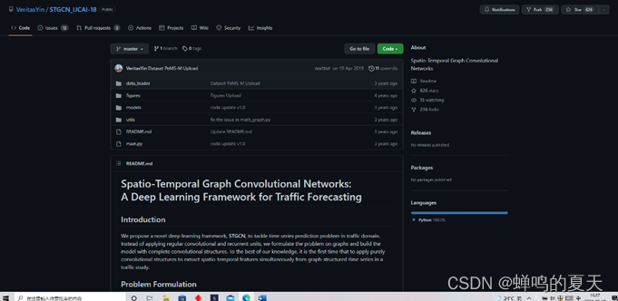
STGCN的环境配置
代码库地址:https://github.com/VeritasYin/STGCN_IJCAI-18

更新最新的地址:
conda config --add channels https://mirrors.tuna.tsinghua.edu.cn/anaconda/pkgs/main/
conda config --add channels https://mirrors.tuna.tsinghua.edu.cn/anaconda/pkgs/free/
conda config --add channels https://mirrors.tuna.tsinghua.edu.cn/anaconda/cloud/msys2/
conda config --add channels http://mirrors.tuna.tsinghua.edu.cn/anaconda/cloud/pytorch/
conda config --add channels http://mirrors.tuna.tsinghua.edu.cn/anaconda/cloud/conda-forge/
conda config --add channels http://mirrors.tuna.tsinghua.edu.cn/anaconda/cloud/bioconda/
conda config --add channels https://mirror.tuna.tsinghua.edu.cn/anaconda/pkgs/pro
conda config --add channels https://mirror.tuna.tsinghua.edu.cn/anaconda/pkgs/r
conda config --add channels http://mirrors.aliyun.com/pypi/simple/
创建新的虚拟环境:
conda create -n py36ts19 python=3.6
激活环境:
conda activate py36ts19
安装tensorflow:
pip install scrapy -i https://pypi.tuna.tsinghua.edu.cn/simple tensorflow==1.9 pip==21.3.1
pip install scrapy -i https://pypi.tuna.tsinghua.edu.cn/simple tensorflow-gpu==1.9 pip==21.3.1
安装NumPy:
pip install -U numpy==1.15 -i https://pypi.tuna.tsinghua.edu.cn/simple
安装SciPy:
pip install -U scipy==1.1.0 -i https://pypi.tuna.tsinghua.edu.cn/simple
安装Pandas:
pip install -U pandas==0.23 -i https://pypi.tuna.tsinghua.edu.cn/simple
克隆项目:
git clone https://github.com/VeritasYin/STGCN_IJCAI-18.git
安装cuda和cudnn:
conda install cudatoolkit=9.0
conda install cudnn=7
退出环境:
conda deactivate
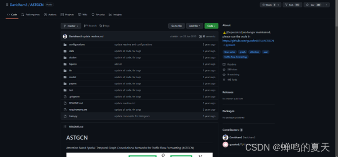
ASTGCN、STSGCN和STFGNN的环境配置
代码库地址:
ASTGCN:https://github.com/Davidham3/ASTGCN
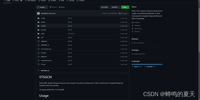
STSGCN:https://github.com/Davidham3/STSGCN
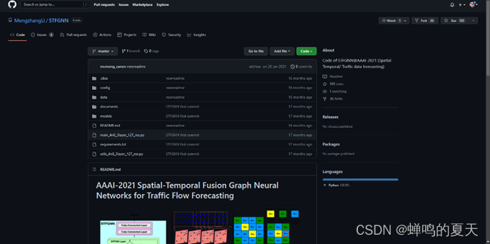
STFGNN:https://github.com/MengzhangLI/STFGNN
他们都推荐用docker,但是docker-gup只能在Liunx环境上安装,所以我没有用docker来快速安装,还是用conda:
conda create -n  mxnet_envs python=3.6
conda remove -n mxnet_envs --all
conda activate mxnet_envs
conda install cudatoolkit=10.0.130
conda install cudnn=7.3.1
pip install mxnet-cu100 -i https://pypi.tuna.tsinghua.edu.cn/simple
pip install -U pytest
pip install -i https://pypi.tuna.tsinghua.edu.cn/simple graphviz==0.8.4
conda deactivate
数据集
数据集的收集
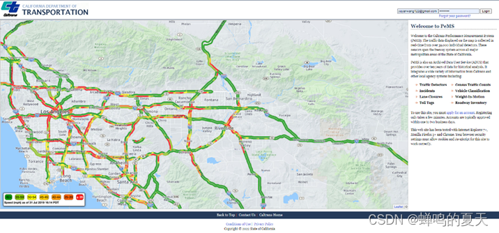
到这个网址https://pems.dot.ca.gov/?dnode=Clearinghouse上注册登录(注意只能使用国外邮箱哦。)
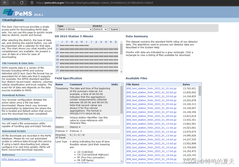
时间序列,选择Station 5-Minute、District X,下面就会有01年到22年的每个月每日的交通流量数据:
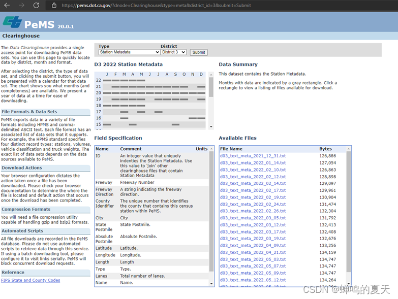
空间位置数据,选择Station metadata,选择对应地区的对应月份就可以得到对应的传感器空间位置数据集:
此页面旁边也有对数据的描述:
对于时间序列的描述:
特征描述Timestamp摘要间隔开始的日期和时间。例如,时间 08:00:00 表示聚合包含在 08:00:00 和 08:04:59 之间收集的度量值。请注意,对于五分钟的聚合,第二个值始终为 0。格式为 MM/DD/YYYY HH24:MI:SS。Station唯一的工作站标识符。使用此值可与元数据文件交叉引用。District#区Freeway#高速公路Direction of Travel前往路线N \S \E \WLane Type指示车道类型的字符串。可能的值(及其含义为:CD (Coll/Dist);CH(常规公路);FF (Fwy-Fwy 连接器);FR(下坡道);高压(HOV);ML (主线);OR(斜坡上)Station Length车站覆盖的航段长度(以英里/公里为单位)。Samples所有车道收到的样本总数。% Observed在此位置观察到的单个车道点的百分比(例如,not imputed)。Total Flow5 分钟内所有车道的流量总和。请注意,基本的 5 分钟汇总会根据从控制器接收到的良好样本数对流程进行标准化。Veh/5-minAvg Occupancy5 分钟内所有车道的平均占用率以介于 0 和 1 之间的十进制数表示。%Avg Speed所有车道上 5 分钟内的流量加权平均速度。如果流量为 0,则为 5 分钟工位速度的数学平均值。MphLane N SamplesN通道收到的合格样品数(范围从 1 到该位置的通道数)Lane N Flow通道N在 5 分钟内的总流量由良好样品的数量归一化Veh/5-minLane N Avg Occ车道N的平均占用率表示为介于 0 和 1 之间的十进制数。(N的范围从 1 到该位置的车道数)%Lane N Avg Speed车道 N 速度的流量加权平均值。如果流量为 0,则为 5 分钟车道速度的数学平均值。N 范围从 1 到车道数MphLane N Observed1 表示观测到的数据,0 表示插补的数据。
对于空间序列的描述:
特征描述ID一个整数值,用于唯一缩进工作站元数据。使用此值可以”加入”包含电台元数据的其他信息交换所文件Freeway高速公路号码Freeway Direction指示高速公路方向的字符串County Identifie标识 PeMS 中包含此站的唯一编号。City城市State Postmile国家里程Absolute Postmile绝对里程Latitude经度Longitude纬度Length长度Type类型Lanes车道总数Name名字User IDs[1-4]用户输入的字符串标识符
; 数据集的预处理
数据集的预处理的整体思路就是:

时间序列和空间序列要保留的特征加粗了:
Station 5-Minute: Timestamp、Station、District#、Freeway#、Direction of Travel、Lane Type、Station Length、Samples、% Observed、 Total Flow、Avg Occupancy、Avg Speed、Lane N Samples、Lane N Flow、Lane N Avg Occ、Lane N Avg Speed、Lane N Observed
Station metadata: ID、 Freeway、Freeway Direction、County Identifie、City、State Postmile、 Absolute Postmile、Latitude、Longitude、Length、Type、Lanes、Name、User IDs[1-4]
STGCN只用了一个特征值speed,ASTGCN、STSGCN和STFGNN的特征向量是flow、occupancy和speed。所以评价指标的大小会有差异哦。
import csv
from os import listdir
import pandas as pd
import numpy as np
from geopy.distance import geodesic

num_station = 50

num_days = 31

dir = '下载的数据集存放的文件夹'

for filename in listdir(dir):

    if filename.endswith('.csv'):

        data = pd.read_csv(下载的数据集存放的文件夹' + filename, header=None)

        data_station = data.iloc[:, 1]
        station_nums = np.array(data_station)
        after_enumerate = enumerate(station_nums)
        li = []

        for station_index, station_num in after_enumerate:
            if station_index % 10 == 0:
                print(station_index, station_num)
            if station_num > 715974:
                li.append(station_index)
        data_new = data.drop(labels=li, axis=0).loc[:, [0, 1, 9, 10, 11]]
        data_new.to_csv('aggregation.csv', mode='a', index=None, header=None)
        print(filename + ' is done!')

datas = pd.read_csv('aggregation.csv', header=None)
datas = datas.interpolate(method='values')

v_value = np.zeros((288 * num_days, num_station))

fos = np.zeros((288 * num_days, num_station, 3))
for i in range(0, 288 * num_days):
    for j in range(0, num_station):
        v_value[i][j] = datas.loc[i * num_station + j, 2]
        fos[i][j][0] = datas.loc[i * num_station + j, 2]
        fos[i][j][1] = datas.loc[i * num_station + j, 3]
        fos[i][j][2] = datas.loc[i * num_station + j, 4]

new_data_v = pd.DataFrame(v_value)
new_data_v.to_csv('PeMSD7_V_50.csv', index=None, header=None)
np.savez('PeMS22_07.npz', data=fos)
print('时间序列片变换完毕!')

txt_file = r"D:\BYSJ\pems77_07\d7_sation.txt"
csv_file = r"d07_meta_2022_03.csv"

csvFile = open(csv_file, 'w', newline='', encoding='utf-8')
writer = csv.writer(csvFile)
csvRow = []

f = open(txt_file, 'r', encoding='utf-8')
for line in f:
    csvRow = line.split()
    writer.writerow(csvRow)

f.close()
csvFile.close()

data = pd.read_csv('d07_meta_2022_03.csv')

sid = data.iloc[:, 0]

fwy = data.iloc[:, 1]

apm = data.iloc[:, 7]

lat = data.iloc[:, 8]

lon = data.iloc[:, 9]

datas = np.zeros((num_station, num_station))
for i in range(0, num_station):
    for j in range(0, num_station):
        datas[i][j] = geodesic((lat[i], lon[i]), (lat[j], lon[j])).m
weight_csv = pd.DataFrame(datas)

weight_csv.to_csv('PeMSD7_W_50.csv', header=None, index=None)

cost = np.zeros((num_station, num_station))

cost_arr = []
for i in range(0, num_station):
    for j in range(0, i):
        if i != j and fwy[i] == fwy[j]:
            cost[i][j] = abs(apm[i] - apm[j])

for i in range(0, num_station):
    min_cost = 3000
    min_index = 0
    for j in range(0, num_station):
        if cost[i][j] != 0 and cost[i][j] < min_cost:
            min_index = j
            min_cost = cost[i][j]
    if i != min_index and min_cost != 3000:
        cost_arr.append([i, min_index, min_cost * 1.6093])
dis_csv = pd.DataFrame(cost_arr, columns=['from', 'to', 'cost'])
dis_csv.to_csv('d07_distance.csv')
print('空间序列片变换完毕!')
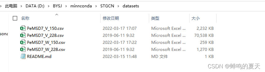
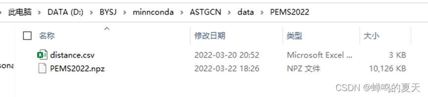
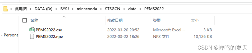
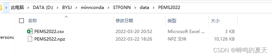
我们把处理好的数据集放在这些文件夹下:
模型的训练
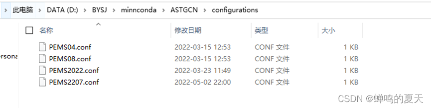
训练ASTGCN、STSGCN、STFGNN模型前要先写配置文件,比如ASTGCN模型的配置文件:
[Data]
adj_filename = data/PEMS2022/distance.csv
graph_signal_matrix_filename = data/PEMS2022/PEMS2022.npz
num_of_vertices = 150
points_per_hour = 12
num_for_predict = 12

[Training]
model_name = ASTGCN
ctx = gpu-0
optimizer = adam
learning_rate = 0.001
epochs = 70
batch_size = 16
num_of_weeks = 1
num_of_days = 1
num_of_hours = 3
K = 3
merge = 0
prediction_filename = ASTGCN_prediction_2022
params_dir = experiment2
STGCN模型可以在main.py中修改默认配置,也可以在输入命令时传入配置:
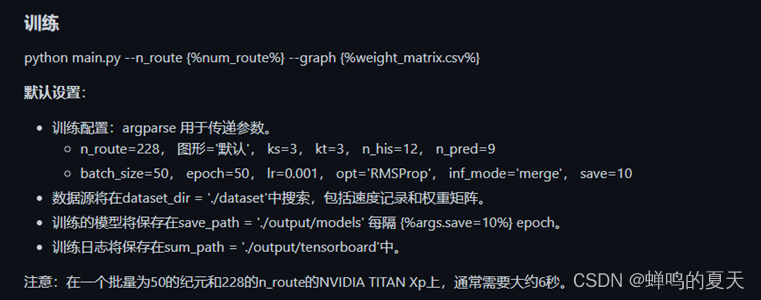
STGCN:(py36ts19)python main.py --n_route 150 --graph  D:\BYSJ\minnconda\STGCN_IJCAI-18\dataset/PeMSD7_W_150.csv --epoch 70
ASTGCN:(mxnet_envs) python main.py --config configurations/PEMS2207.conf --force True
STSGCN:(mxnet_envs) python main.py --config config/PEMS2022/individual_GLU_mask_emb.json
STFGNN:(mxnet_envs) python main_4n0_3layer_12T_res.py --config config/PEMS2022/individual_3layer_12T.json
重复十次训练的代码:
import os, re

def execCmd(cmd):
    r = os.popen(cmd)
    text = r.read()
    r.close()
    return text

def writeFile(filename, data):
    f = open(filename, "a")
    f.write(data)
    f.close()

if __name__ == '__main__':
    for i in range(10):
        print(i)
        cmd = "python main.py"
        result = execCmd(cmd)
        filename = "存放输出的文件位置"
        writeFile(filename, result)
数据集
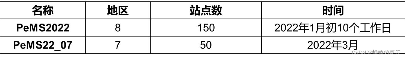
我自己收集处理两个数据集,分别命名为PeMS2022和PeMS22_07
戳这里下载哦。提取码:qbh6
Original: https://blog.csdn.net/yukiaustin/article/details/125122206
Author: 蝉鸣的夏天
Title: STGCN、ASTGCN、STSGCN、STFGNN模型的对比实验操作步骤
原创文章受到原创版权保护。转载请注明出处:https://www.johngo689.com/627319/
转载文章受原作者版权保护。转载请注明原作者出处!