Extended Physics-InformedNeural Networks论文详解

作者

* Ameya D. Jagtap1,∗ and George Em Karniadakis1,2

期刊

* Communications in Computational Physics

日期

* 2020

代码

* 代码链接

1 摘要

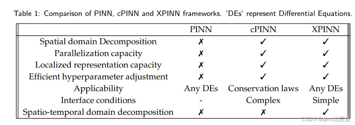
提出了更灵活分解域的XPINN方法，比cPINN区域分解更灵活，而且使用与所有方程。

2 背景

cPINN是通过区域分解，每个区域使用小的网络进行训练，使得求解时不同区域能够并行计算。论文提出的XPINN具有cPINN的区域分解的优势，同时还有以下优势

* Generalized space-time domain decomposition，XPINN公式提供了高度不规则的、凸/非凸的时空域分解，由于这样的分解XPINN公式提供了高度不规则的、凸/非凸的时空域分解

* XPINN公式提供了高度不规则的、凸/非凸的时空域分解

* 简单中间条件，在XPINN中，对于任意形状的界面来说，界面条件非常简单，不需要法线方向，因此，所提出的方法可以很容易地扩展到任何复杂的几何形状，甚至是更高维度的几何形状。

精确求解复杂的方程组，特别是高维方程组已经成为科学计算的最大挑战之一。XPINN的优点使其成为适合进行此类高维复杂模拟的候选对象，而这个高维模拟通常需要大量的训练成本的。

3 XPINN方法

描述：

* Subdomains ：子域Ω q , q = 1 , 2 , ⋯ N s d \Omega_{q}, q=1,2, \cdots N_{s d}Ωq ​,q =1 ,2 ,⋯N s d ​是整个计算域Ω \Omega Ω的非重叠子域，满足Ω = ⋃ q = 1 N s d Ω q \Omega=\bigcup_{q=1}^{N_{s d}} \Omega_{q}Ω=⋃q =1 N s d ​​Ωq ​和Ω i ∩ Ω j = ∂ Ω i j , i ≠ j \Omega_{i} \cap \Omega_{j}=\partial \Omega_{i j}, i \neq j Ωi ​∩Ωj ​=∂Ωij ​,i =j表示分解域的个数，子域的相交仅仅是在边界∂ Ω i j \partial \Omega_{i j}∂Ωij ​

* Interface ：表示两个或者多个子域的共同边界对应的子网（sub-Nets）之间互通

* sub-Net：子PINN是指每个子域中使用的具有自己的一组优化超参数的个体PINN

* Interface Conditions: 这些条件用于将分解的子域连接在一起，从而得到完全域上的控制偏微分方程的解,根据控制方程的性质，一个或多个界面条件可以应用在共同界面上，如解连续性、通量连续性等

上图中X就是求解域，黑色实线表示区域的边界，黑色虚线表示interface。XPINN的基本interface条件包括强形式的连续性条件和在共同interface上强制不同子网给出的平均解。cPINN文中提到，为了稳定性，没有必要加平均解的条件，但实验也表明了会加快收敛速度。XPINN具有cPINN的所有优点，如并行化能力、大的表示能力、优化方法、激活函数、网络深度或宽度等超参数的高效选择。与cPINN不同，XPINN可以用于求解任何类型的偏微分方程，而不一定是守恒定律。在XPINN情况下，采用法向通量连续性条件不需要找到法向。这大大降低了算法的复杂性，特别是在具有复杂领域的大规模问题以及移动界面问题。

第q t h q^{t h}q t h个子域的神经网络输出定义为

u Θ ~ q ( z ) = N L ( z ; Θ ~ q ) ∈ Ω q , q = 1 , 2 , ⋯ , N s d u_{\tilde{\mathbf{\Theta}}{q}}(\mathbf{z})=\mathcal{N}^{L}\left(\mathbf{z} ; \tilde{\mathbf{\Theta}}{q}\right) \in \Omega_{q}, \quad q=1,2, \cdots, N_{s d}u Θ~q ​​(z )=N L (z ;Θ~q ​)∈Ωq ​,q =1 ,2 ,⋯,N s d ​

最终解定义为

u Θ ~ ( z ) = ∑ q = 1 N s d u Θ ~ q ( z ) ⋅ 1 Ω q ( z ) u_{\tilde{\mathbf{\Theta}}}(\mathbf{z})=\sum_{q=1}^{N_{s d}} u_{\tilde{\mathbf{\Theta}}{q}}(\mathbf{z}) \cdot \mathbb{1}{\Omega_{q}}(\mathbf{z})u Θ~​(z )=∑q =1 N s d ​​u Θ~q ​​(z )⋅1 Ωq ​​(z )

其中

1 Ω q ( z ) : = { 0 if z ∉ Ω q 1 if z ∈ Ω q \ Common interface in the q t h subdomain 1 S if z ∈ Common interface in the q t h subdomain \mathbb{1}{\Omega{q}}(\mathbf{z}):=\left{\begin{array}{ll} 0 & \text { if } \mathbf{z} \notin \Omega_{q} \ 1 & \text { if } \mathbf{z} \in \Omega_{q} \backslash \text { Common interface in the } q^{t h} \text { subdomain } \ \frac{1}{\mathcal{S}} & \text { if } \mathbf{z} \in \text { Common interface in the } q^{t h} \text { subdomain } \end{array}\right.1 Ωq ​​(z ):=⎩⎨⎧​0 1 S 1 ​​if z ∈/Ωq ​if z ∈Ωq ​\Common interface in the q t h subdomain if z ∈Common interface in the q t h subdomain ​

S S S表示S表示沿公共界面相交的子域数量

3.1 正、逆问题子域的损失函数

(1)正问题

在q t h q^{t h}q t h子域的{ x u q ( i ) } i = 1 N u q , { x F q ( i ) } i = 1 N F q and { x I q ( i ) } i = 1 N I q \left{\mathbf{x}{u{q}}^{(i)}\right}{i=1}^{N{u q}},\left{\mathbf{x}{F{q}}^{(i)}\right}{i=1}^{N{F q}} \text { and }\left{\mathbf{x}{I{q}}^{(i)}\right}{i=1}^{N{I q}}{x u q ​(i )​}i =1 N u q ​​,{x F q ​(i )​}i =1 N Fq ​​and {x I q ​(i )​}i =1 N I q ​​表示training, residual, and the common interface points。N u q , N F q a n d N I q N_{u_{q}}, N_{F_{q}} and N_{I q}N u q ​​,N F q ​​an d N I q ​分别代表对应的点的个数，每个子域使用一个PINN，u q = u Θ ~ t u_{q}=u_{\tilde{\Theta}{t}}u q ​=u Θ~t ​​,第q t h q^{t h}q t h个子域损失函数定义为

J ( Θ ~ q ) = W u q MSE ⁡ u q ( Θ ~ q ; { x u q ( i ) } i = 1 N u q ) + W F q MSE ⁡ F q ( Θ ~ q ; { x F q ( i ) } i = 1 N F q ) + W I q MSE ⁡ u a v g ( Θ ~ q ; { x I q ( i ) } i = 1 N I q ) ⏟ Interface condition + W I F q MSE ⁡ R ( Θ ~ q ; { x I q ( i ) } i = 1 N I q ) ⏟ Interface condition + Additional Interface Condition’s ⏟ Optional \begin{aligned} \mathcal{J}\left(\tilde{\mathbf{\Theta}}{q}\right)=& W_{u_{q}} \operatorname{MSE}{u{q}}\left(\tilde{\mathbf{\Theta}}{q} ;\left{\mathbf{x}{u_{q}}^{(i)}\right}{i=1}^{N{u q}}\right)+W_{\mathcal{F}{q}} \operatorname{MSE}{\mathcal{F}{q}}\left(\tilde{\boldsymbol{\Theta}}{q} ;\left{\mathbf{x}{F{q}}^{(i)}\right}{i=1}^{N{F q}}\right) \ &+W_{I_{q}} \underbrace{\operatorname{MSE}{u{a v g}}\left(\tilde{\boldsymbol{\Theta}}{q} ;\left{\mathbf{x}{I_{q}}^{(i)}\right}{i=1}^{N{I q}}\right)}{\text {Interface condition }}+W{I_{\mathcal{F}{q}}} \underbrace{\operatorname{MSE}{\mathcal{R}}\left(\tilde{\boldsymbol{\Theta}}{q} ;\left{\mathbf{x}{I_{q}}^{(i)}\right}{i=1}^{N{I q}}\right)}{\text {Interface condition }} \ &+\underbrace{\text { Additional Interface Condition’s }}{\text {Optional }} \end{aligned}J (Θ~q ​)=​W u q ​​MSE u q ​​(Θ~q ​;{x u q ​(i )​}i =1 N u q ​​)+W F q ​​MSE F q ​​(Θ~q ​;{x F q ​(i )​}i =1 N Fq ​​)+W I q ​​Interface condition MSE u a vg ​​(Θ~q ​;{x I q ​(i )​}i =1 N I q ​​)​​+W I F q ​​​Interface condition MSE R ​(Θ~q ​;{x I q ​(i )​}i =1 N I q ​​)​​+Optional Additional Interface Condition’s ​​​

W u q , W F q , W I F q and W I q W_{u_{q}}, W_{\mathcal{F}{q}}, W{I_{\mathcal{F}{q}}} \text { and } W{I_{q}}W u q ​​,W F q ​​,W I F q ​​​and W I q ​​代表不同损失的参数,

MSE ⁡ u q ( Θ ~ q ; { x u q ( i ) } i = 1 N u q ) = 1 N u q ∑ i = 1 N u q ∣ u ( i ) − u Θ ~ q ( x u q ( i ) ) ∣ 2 MSE ⁡ F q ( Θ ~ q ; { x F q ( i ) } i = 1 N F q ) = 1 N F a ∑ i = 1 N F q ∣ F Θ ~ q ( x F q ( i ) ) ∣ 2 \begin{array}{l} \operatorname{MSE}{u{q}}\left(\tilde{\mathbf{\Theta}}{q} ;\left{\mathbf{x}{u_{q}}^{(i)}\right}{i=1}^{N{u q}}\right)=\frac{1}{N_{u_{q}}} \sum_{i=1}^{N_{u q}}\left|u^{(i)}-u_{\tilde{\mathbf{\Theta}}{q}}\left(\mathbf{x}{u_{q}}^{(i)}\right)\right|^{2} \ \operatorname{MSE}{\mathcal{F}{q}}\left(\tilde{\mathbf{\Theta}}{q} ;\left{\mathbf{x}{F_{q}}^{(i)}\right}{i=1}^{N{F q}}\right)=\frac{1}{N_{F_{a}}} \sum_{i=1}^{N_{F q}}\left|\mathcal{F}{\tilde{\mathbf{\Theta}}{q}}\left(\mathbf{x}{F{q}}^{(i)}\right)\right|^{2} \end{array}MSE u q ​​(Θ~q ​;{x u q ​(i )​}i =1 N u q ​​)=N u q ​​1 ​∑i =1 N u q ​​∣∣​u (i )−u Θ~q ​​(x u q ​(i )​)∣∣​2 MSE F q ​​(Θ~q ​;{x F q ​(i )​}i =1 N Fq ​​)=N F a ​​1 ​∑i =1 N Fq ​​∣∣​F Θ~q ​​(x F q ​(i )​)∣∣​2 ​

MSE ⁡ u a v g ( Θ ~ q ; { x I q ( i ) } i = 1 N I q ) = ∑ ∀ q + ( 1 N I q ∑ i = 1 N I q ∣ u Θ ~ q ( x I q ( i ) ) − { { u Θ ~ q ( x I q ( i ) ) } } ∣ 2 ) MSE ⁡ R ( Θ ~ q ; { x I q ( i ) } i = 1 N I q ) = ∑ ∀ q + ( 1 N I q ∑ i = 1 N I q ∣ F Θ ~ q ( x I q ( i ) ) − F Θ ~ q + ( x I q ( i ) ) ∣ 2 ) \begin{array}{l} \operatorname{MSE}{u{a v g}}\left(\tilde{\mathbf{\Theta}}{q} ;\left{\mathbf{x}{I_{q}}^{(i)}\right}{i=1}^{N{I q}}\right)=\sum_{\forall q^{+}}\left(\frac{1}{N_{I_{q}}} \sum_{i=1}^{N_{I_{q}}}\left|u_{\tilde{\mathbf{\Theta}}{q}}\left(\mathbf{x}{I_{q}}^{(i)}\right)-\left{\left{u_{\tilde{\mathbf{\Theta}}{q}}\left(\mathbf{x}{I_{q}}^{(i)}\right)\right}\right}\right|^{2}\right) \ \operatorname{MSE}{\mathcal{R}}\left(\tilde{\mathbf{\Theta}}{q} ;\left{\mathbf{x}{I{q}}^{(i)}\right}{i=1}^{N{I q}}\right)=\sum_{\forall q^{+}}\left(\frac{1}{N_{I_{q}}} \sum_{i=1}^{N_{I_{q}}}\left|\mathcal{F}{\tilde{\mathbf{\Theta}}{q}}\left(\mathbf{x}{I{q}}^{(i)}\right)-\mathcal{F}{\tilde{\Theta}{q^{+}}}\left(\mathbf{x}{I{q}}^{(i)}\right)\right|^{2}\right) \end{array}MSE u a vg ​​(Θ~q ​;{x I q ​(i )​}i =1 N I q ​​)=∑∀q +​(N I q ​​1 ​∑i =1 N I q ​​​∣∣​u Θ~q ​​(x I q ​(i )​)−{{u Θ~q ​​(x I q ​(i )​)}}∣∣​2 )MSE R ​(Θ~q ​;{x I q ​(i )​}i =1 N I q ​​)=∑∀q +​(N I q ​​1 ​∑i =1 N I q ​​​∣∣​F Θ~q ​​(x I q ​(i )​)−F Θ~q +​​(x I q ​(i )​)∣∣​2 )​

最后两项代表着interface 条件损失,第四项是在子域q q q和q + q^{+}q +的两个不同网络的残差连续条件,q + q^{+}q +代表q q q的领域MSER和M S E u a v g MSE_{uavg}MS E u a vg ​，都定义在所有相邻的子域,上式子中{ { u Θ ~ q } } = u avg : = u Θ ~ q + u Θ ~ q + 2 \left{\left{u_{\tilde{\mathbf{\Theta}}{q}}\right}\right}=u{\text {avg }}:=\frac{u_{\tilde{\mathbf{\Theta}}{q}}+u{\tilde{\mathbf{\Theta}}_{q^{+}}}}{2}{{u Θ~q ​​}}=u avg ​:=2 u Θ~q ​​+u Θ~q +​​​(假设在公共界面上只有两个子域相交)，additional interface conditions，例如flux continuity ，c k c^{k}c k也能根据PDE的类型以及interface 方向被加损失中。

remark：

* interface conditions 的类型决定了整个接口的解的正则性，从而影响收敛速度。在interface上的解是足够连续的，从而满足其控制PDE

* 足够多的interface point去连接子域，这对于算法的收敛很重要，特别是对于internal

对于逆问题:

J ( Θ ~ q , λ ) = W u q MSE ⁡ u q ( Θ ~ q , λ ; { x u q ( i ) } i = 1 N u q ) + W F q MSE ⁡ F q ( Θ ~ q , λ ; { x u q ( i ) } i = 1 N u q ) + W I q { MSE ⁡ u a v g ( Θ ~ q , λ ; { x I q ( i ) } i = 1 N I q ) + MSE ⁡ λ ( θ ~ q , λ ; { x I q ( i ) } i = 1 N I q ) } ⏟ Interface condition’s + W I F q MSE ⁡ R ( Θ ~ q , λ ; { x I q ( i ) } i = 1 N I q ) ⏟ Intarf + Additional Interface Condition’s ⏟ Optional \begin{aligned} \mathcal{J}\left(\tilde{\mathbf{\Theta}}{q}, \lambda\right)=& W{u_{q}} \operatorname{MSE}{u{q}}\left(\tilde{\boldsymbol{\Theta}}{q}, \lambda ;\left{\mathbf{x}{u_{q}}^{(i)}\right}{i=1}^{N{u_{q}}}\right)+W_{\mathcal{F}{q}} \operatorname{MSE}{\mathcal{F}{q}}\left(\tilde{\boldsymbol{\Theta}}{q}, \lambda ;\left{\mathbf{x}{u{q}}^{(i)}\right}{i=1}^{N{u_{q}}}\right) \ &+W_{I_{q}} \underbrace{\left{\operatorname{MSE}{u{a v g}}\left(\tilde{\boldsymbol{\Theta}}{q}, \lambda ;\left{\mathbf{x}{I_{q}}^{(i)}\right}{i=1}^{N{I q}}\right)+\operatorname{MSE}{\lambda}\left(\tilde{\boldsymbol{\theta}}{q}, \lambda ;\left{\mathbf{x}{I{q}}^{(i)}\right}{i=1}^{N{I q}}\right)\right}}{\text {Interface condition’s }} \ &+W{I_{\mathcal{F}{q}}} \underbrace{\operatorname{MSE}{\mathcal{R}}\left(\tilde{\boldsymbol{\Theta}}{q}, \lambda ;\left{\mathbf{x}{I_{q}}^{(i)}\right}{i=1}^{N{I q}}\right)}{\text {Intarf }}+\underbrace{\text { Additional Interface Condition’s }}{\text {Optional }} \end{aligned}J (Θ~q ​,λ)=​W u q ​​MSE u q ​​(Θ~q ​,λ;{x u q ​(i )​}i =1 N u q ​​​)+W F q ​​MSE F q ​​(Θ~q ​,λ;{x u q ​(i )​}i =1 N u q ​​​)+W I q ​​Interface condition’s {MSE u a vg ​​(Θ~q ​,λ;{x I q ​(i )​}i =1 N I q ​​)+MSE λ​(θ~q ​,λ;{x I q ​(i )​}i =1 N I q ​​)}​​+W I F q ​​​Intarf MSE R ​(Θ~q ​,λ;{x I q ​(i )​}i =1 N I q ​​)​​+Optional Additional Interface Condition’s ​​​

其中

MSE ⁡ F q ( Θ ~ q , λ ; { x u q ( i ) } i = 1 N u q ) = 1 N u q ∑ i = 1 N u q ∣ F Θ ~ q ( x u q ( i ) ) ∣ 2 MSE ⁡ λ ( Θ ~ q , λ ; { x I q ( i ) } i = 1 N I q ) = ∑ ∀ q + ( 1 N I q ∑ i = 1 N l q ∣ λ q ( x I q ( i ) ) − λ q + ( x I q ( i ) ) ∣ 2 ) \begin{array}{l} \operatorname{MSE}{\mathcal{F}{q}}\left(\tilde{\boldsymbol{\Theta}}{q}, \lambda ;\left{\mathbf{x}{u_{q}}^{(i)}\right}{i=1}^{N{u_{q}}}\right)=\frac{1}{N_{u_{q}}} \sum_{i=1}^{N_{u_{q}}}\left|\mathcal{F}{\tilde{\mathbf{\Theta}}{q}}\left(\mathbf{x}{u{q}}^{(i)}\right)\right|^{2} \ \operatorname{MSE}{\lambda}\left(\tilde{\mathbf{\Theta}}{q}, \lambda ;\left{\mathbf{x}{I{q}}^{(i)}\right}{i=1}^{N{I q}}\right)=\sum_{\forall q^{+}}\left(\frac{1}{N_{I_{q}}} \sum_{i=1}^{N_{l q}}\left|\lambda_{q}\left(\mathbf{x}{I{q}}^{(i)}\right)-\lambda_{q^{+}}\left(\mathbf{x}{I{q}}^{(i)}\right)\right|^{2}\right) \end{array}MSE F q ​​(Θ~q ​,λ;{x u q ​(i )​}i =1 N u q ​​​)=N u q ​​1 ​∑i =1 N u q ​​​∣∣​F Θ~q ​​(x u q ​(i )​)∣∣​2 MSE λ​(Θ~q ​,λ;{x I q ​(i )​}i =1 N I q ​​)=∑∀q +​(N I q ​​1 ​∑i =1 N lq ​​∣∣​λq ​(x I q ​(i )​)−λq +​(x I q ​(i )​)∣∣​2 )​

其他残差损失与正向损失一样。

Remark：需要注意的是，由于XPINN损失函数的高度非凸性，定位其全局最小值非常难。但是，对于几个局部极小值，损失函数的值是相似的，相应的预测解的精度是相似的。

3.2 优化方法

自动求导

3.3 误差

E app q = ∥ u a q − u q e x ∥ E gen q = ∥ u g q − u a q ∥ E opt q = ∥ u τ q − u g q ∥ \begin{aligned} \mathcal{E}{\text {app }} q &=\left\|u{a_{q}}-u_{q}^{e x}\right\| \ \mathcal{E}{\text {gen }} q &=\left\|u{g_{q}}-u_{a_{q}}\right\| \ \mathcal{E}{\text {opt }} q &=\left\|u{\tau_{q}}-u_{g_{q}}\right\| \end{aligned}E app ​q E gen ​q E opt ​q ​=∥∥​u a q ​​−u q e x ​∥∥​=∥∥​u g q ​​−u a q ​​∥∥​=∥∥​u τq ​​−u g q ​​∥∥​​

分别代表approximation error、 generalization error 以及optimization error.

* u a q = arg ⁡ min ⁡ f ∈ F q ∥ f − u q e x ∥ u_{a_{q}}=\arg \min {f \in F{q}}\left\|f-u_{q}^{e x}\right\|u a q ​​=ar g min f ∈F q ​​∥∥​f −u q e x ​∥∥​是真解u q e x u_{q}^{e x}u q e x ​的近似

* u g q = arg ⁡ min ⁡ Θ ~ q J ( Θ ~ q ) u_{g_{q}}=\arg \min {\tilde{\mathbf{\Theta}}{q}} \mathcal{J}\left(\tilde{\mathbf{\Theta}}{q}\right)u g q ​​=ar g min Θ~q ​​J (Θ~q ​)是全局最优解

* u τ q = arg ⁡ min ⁡ Θ ~ q J ( Θ ~ q ) u{\tau_{q}}=\arg \min {\tilde{\mathbf{\Theta}}{q}} \mathcal{J}\left(\tilde{\mathbf{\Theta}}_{q}\right)u τq ​​=ar g min Θ~q ​​J (Θ~q ​)是子网络训练后得到的解，

最后XPINN的误差可以总结为

E X P I N N : = ∥ u τ − u e x ∥ ≤ ∥ u τ − u g ∥ + ∥ u g − u a ∥ + ∥ u a − u e x ∥ \mathcal{E}{X P I N N}:=\left\|u{\tau}-u^{e x}\right\| \leq\left\|u_{\tau}-u_{g}\right\|+\left\|u_{g}-u_{a}\right\|+\left\|u_{a}-u^{e x}\right\|E XP I NN ​:=∥u τ​−u e x ∥≤∥u τ​−u g ​∥+∥u g ​−u a ​∥+∥u a ​−u e x ∥

其中，( u e x , u τ , u g , u a ) ( z ) = ∑ q = 1 N s d ( u q e x , u τ q , u g q , u a q ) ( z ) ⋅ 1 Ω q ( z ) \left(u^{e x}, u_{\tau}, u_{g}, u_{a}\right)(\mathbf{z})=\sum_{q=1}^{N_{s d}}\left(u_{q}^{e x}, u_{\tau_{q}}, u_{g_{q}}, u_{a_{q}}\right)(\mathbf{z}) \cdot \mathbb{1}{\Omega{q}}(\mathbf{z})(u e x ,u τ​,u g ​,u a ​)(z )=∑q =1 N s d ​​(u q e x ​,u τq ​​,u g q ​​,u a q ​​)(z )⋅1 Ωq ​​(z )

Remark：

* 当估计误差降低（数据拟合更好），泛化误差就会增加，这是一种bias variance trade-off，影响泛化误差的两个主要因素是the number and distribution of residual points

* 优化误差由损失函数的复杂性影响，网络结构深深影响优化误差

; 3.4 XPINN、cPINN，PINN对比

与PINN和cPINN框架相比，XPINN框架有很多优点，但是它也有一个与之前的框架相同的局限性。绝对误差

PDE解决方案,不会低于的水平，这是由于解决高维非凸优化问题所涉及的不准确性，可能会导致糟糕的极小值

Original: https://blog.csdn.net/weixin_45521594/article/details/125926625
Author: pinn山里娃
Title: Extended Physics-InformedNeural Networks论文详解