

Introduction
In this exercise, you will implement linear regression and get to see it work
on data.
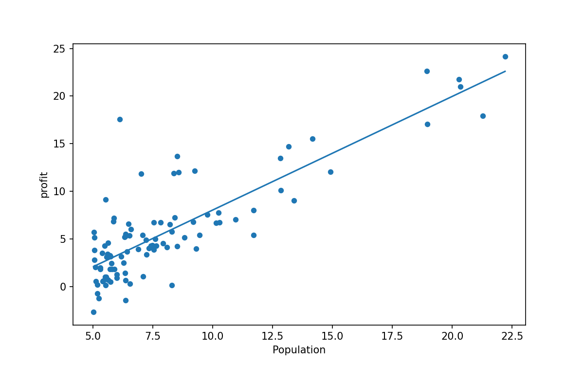
首先,先看看数据是什么样的好进一步分析
import numpy as np
import pandas as pd
import matplotlib.pyplot as plt

path = "data/ex1data1.txt"
data = pd.read_csv(path, header=None, names=['Population', 'profit'])
print(data)
data.plot(kind="scatter", x="Population", y="profit", figsize=(8, 5))
plt.show()
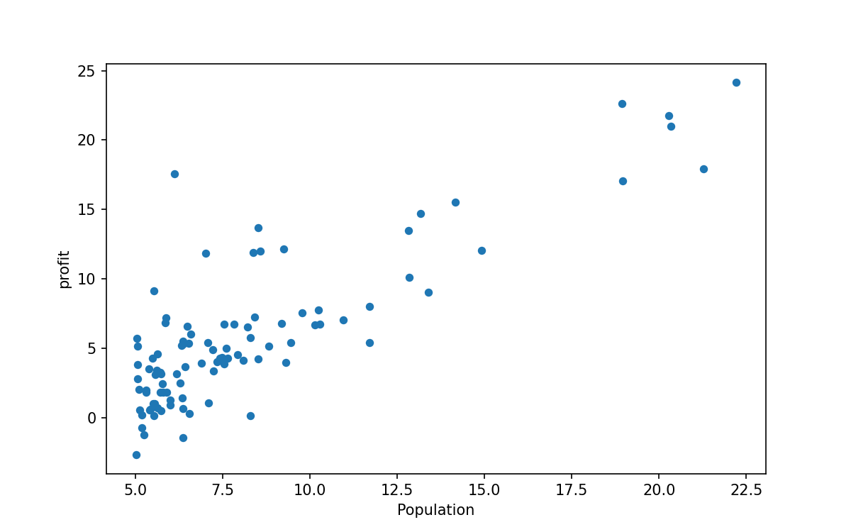

采用线性回归,尽可能准确地预测输出。
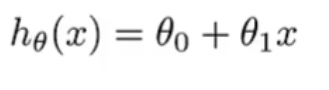
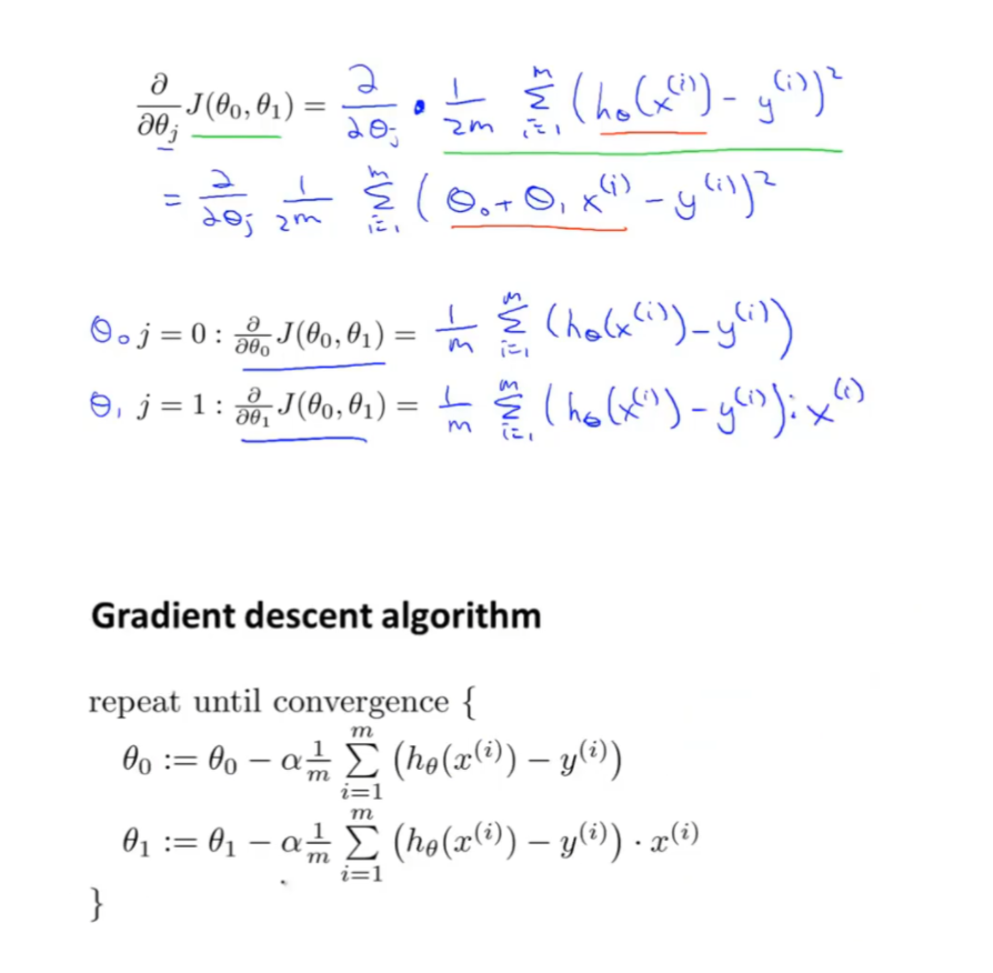
要拟合出一条直线采用均方误差作为损失函数,
我们预测
函数:
损失函数:
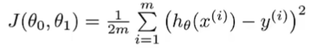
这里均方误差使用1/2m而不是1/m是因为后期梯度下降时,对损失函数求偏导平方求导会出现2,这里乘1/2
会使得后续计算方便
持续更新a于b直到收敛
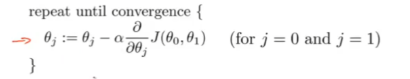
下面就是如何计算偏导数,
def squared_error(a, b):
    res = 0
    for row in data.iterrows():
        population = row[1][0]
        profit = row[1][1]
        res += pow(population*a+b - profit, 2)
    res = 1/(2*data.size)*res
    return res
使得均方误差足够小的a和b即为解,使用梯度下降.
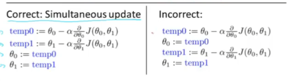
同时更新a和b直到均方误差足够小(凭自己喜好),这里我规定偏导数

达到-9数量级时认为收敛,
附上源码
import numpy as np
import pandas as pd
import matplotlib.pyplot as plt

def squared_error(a, b):
    res = 0
    d_a = 0
    d_b = 0
    for row in data.iterrows():
        population = row[1][0]
        profit = row[1][1]
        res += pow(population*a + b - profit, 2)
        d_a += (population*a + b - profit) * population
        d_b += (population*a + b - profit)
    res *= 1/(2*len(data))
    d_a *= 1/len(data)
    d_b *= 1/len(data)
    print("欧氏距离:", res, "   d_a:", d_a,  "     a:", a)
    return d_a, d_b

def gradient_descent(a, b, alpha):
    d_a, d_b = squared_error(a, b)
    print(type(d_b))
    while abs(d_a) > 10e-9 and abs(d_b) > 10e-9:
        tamp_a = a - alpha * d_a
        tamp_b = b - alpha * d_b
        a = tamp_a
        b = tamp_b
        d_a, d_b = squared_error(a, b)
    return a, b

path = "data/ex1data1.txt"
data = pd.read_csv(path, header=None, names=['Population', 'profit'])
data.plot(kind="scatter", x="Population", y="profit", figsize=(8, 5))

a, b = gradient_descent(0, 0, 0.02)
x = np.linspace(data.Population.min(), data.Population.max(), 100)
y = a*x + b
plt.plot(x, y)
plt.show()
结果如下
Original: https://blog.csdn.net/qq_20180171/article/details/123972082
Author: Cun kou
Title: 吴恩达机器学习作业一
原创文章受到原创版权保护。转载请注明出处:https://www.johngo689.com/618303/
转载文章受原作者版权保护。转载请注明原作者出处!