

目录
1、数据集准备
本文使用sklearn的鸢尾花数据。
sklearn.datasets.load_iris(*, return_X_y=False, as_frame=False)
Iris数据集是常用的分类实验数据集,由Fisher, 1936收集整理。Iris也称鸢尾花卉数据集,是一类多重变量分析的数据集。数据集包含150个数据样本,分为3类,每类50个数据,每个数据包含4个属性(分别是:花萼长度,花萼宽度,花瓣长度,花瓣宽度)。可通过这4个属性预测鸢尾花卉属于(Setosa,Versicolour,Virginica)三个种类的鸢尾花中的哪一类。
Iris里有两个属性iris.data,iris.target。data是一个矩阵,每一列代表了萼片或花瓣的长宽,一共4列,每一列代表某个被测量的鸢尾植物,一共有150条记录。
1.1 导入包
import pandas as pd
import numpy as np
from sklearn.datasets import load_iris
import matplotlib.pyplot as plt
1.2 加载数据
iris = load_iris()用来加载数据
df['label'] = iris.target划分数据的标签
这里我们只取花萼长度,花萼宽度,花瓣长度,花瓣宽度为属性
df.columns = ['sepal length', 'sepal width', 'petal length', 'petal width', 'label']
iris = load_iris()
df = pd.DataFrame(iris.data, columns=iris.feature_names)
df['label'] = iris.target
df.columns = ['sepal length', 'sepal width', 'petal length', 'petal width', 'label']
df.label.value_counts()
1.3 原始数据可视化
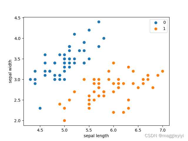
按照花萼长度,花萼宽度进行可视化数据划分,0-49为0类,50-99为1类。
plt.scatter(df[:50]['sepal length'], df[:50]['sepal width'], label='0')
plt.scatter(df[50:100]['sepal length'], df[50:100]['sepal width'], label='1')
plt.xlabel('sepal length')
plt.ylabel('sepal width')

1.4划分数据集和标签
由于感知机是二分类的划分,因此本次选取鸢尾花的前两个类型进行训练预测。也就是前100个数据(0-99)。并且输入维度控制为2维,所以选取第0、1列特征。最后一列是target。并且按照感知机原理将y值设为-1、1的二分类。
data = np.array(df.iloc[:100, [0, 1,-1]])
X, y = data[:, :-1], data[:, -1]
y = np.array([1 if i == 1 else -1 for i in y])
2、感知机实现
2.1 初始化w、b、以及步长
    def __init__(self):
        self.w = np.ones(len(data[0]) - 1, dtype=np.float32)
        self.b = 0
        self.l_rate = 0.1
2.2 设计激活函数
    def sign(self, x, w, b):
        y = np.dot(x, w) + b
        return y
2.3 随机梯度下降
    def fit(self, X_train, y_train):
        is_wrong = False
        while not is_wrong:
            wrong_count = 0
            for d in range(len(X_train)):
                X = X_train[d]
                y = y_train[d]
                if y * self.sign(X, self.w, self.b)
2.4 实现
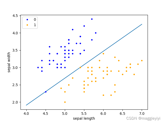
将上述类实现,并可视化展示
二分类线性函数用
x_points = np.linspace(4, 7, 10) y_ = -(perceptron.w[0] * x_points + perceptron.b) / perceptron.w[1] plt.plot(x_points, y_)
其中:y_ = -(perceptron.w[0] * x_points + perceptron.b) / perceptron.w[1]
可以理解为已知法向量和x以及截距b求y的值。
perceptron = Model()
perceptron.fit(X, y)
x_points = np.linspace(4, 7, 10)
y_ = -(perceptron.w[0] * x_points + perceptron.b) / perceptron.w[1]
plt.plot(x_points, y_)
#
plt.plot(data[:50, 0], data[:50, 1], 'bo', color='blue', label='0')
plt.plot(data[50:100, 0], data[50:100, 1], 'bo', color='orange', label='1')
plt.xlabel('sepal length')
plt.ylabel('sepal width')
plt.legend()
plt.show()
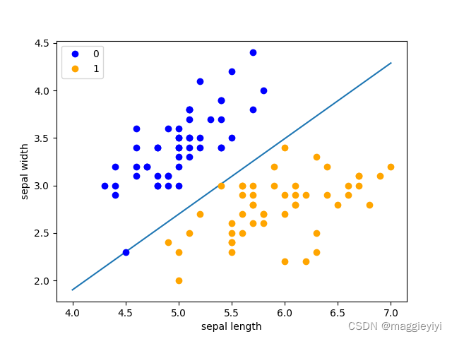
3、检验
利用sklearn自带的感知机函数进行检验
from sklearn.linear_model import Perceptron

In[13]:

clf =  Perceptron(fit_intercept=True, max_iter=1000, shuffle=True, eta0=0.1, tol=None)
clf.fit(X, y)

In[14]:

Weights assigned to the features.

print(clf.coef_)

In[15]:

截距 Constants in decision function.

print(clf.intercept_)

In[16]:

x_ponits = np.arange(4, 8)
y_ = -(clf.coef_[0][0] * x_ponits + clf.intercept_) / clf.coef_[0][1]
plt.plot(x_ponits, y_)

plt.plot(data[:50, 0], data[:50, 1], 'bo', color='blue', label='0')
plt.plot(data[50:100, 0], data[50:100, 1], 'bo', color='orange', label='1')
plt.xlabel('sepal length')
plt.ylabel('sepal width')
plt.legend()
plt.show()
Original: https://blog.csdn.net/maggieyiyi/article/details/125553011
Author: maggieyiyi
Title: 感知机python代码实现
原创文章受到原创版权保护。转载请注明出处:https://www.johngo689.com/614384/
转载文章受原作者版权保护。转载请注明原作者出处!