

本系列所有的代码和数据都可以从陈强老师的个人主页上下载:Python数据程序
参考书目:陈强.机器学习及Python应用. 北京:高等教育出版社, 2021.
本系列基本不讲数学原理,只从代码角度去让读者们利用最简洁的Python代码实现机器学习方法。
本章开始集成学习模型。集成学习的方法在实际问题上表现效果都很好,因为它聚集了很多分类器效果,集成学习的模型一般都被称为’树模型’,因为都是很多很多很多决策树一起估计出来的。随机森林也是这名字的由来。首先要介绍随机森林起源的bagging(袋装法)算法,bagging和后面的boosting区别在于,bagging是装袋了,每个小的估计器之间不相关。而boosting则是每个小估计器之间都相关。bagging在计量里面称为自助法,就是把样本进行很多次重采样,然后分别用不同的估计器去估计,然后再取平均。而随机森林改进的位置在于,每个小分类器之间采用的特征不一样,这样可以降低估计器之间的相关性,虽然可能增大偏差,但也可以更大幅度减少方差。
Bagging的Python案例
首先导入包和数据,采用非线性的数据mcycle
import numpy as np
import pandas as pd
import matplotlib.pyplot as plt
import seaborn as sns
from sklearn.model_selection import train_test_split
from sklearn.model_selection import KFold, StratifiedKFold
from sklearn.model_selection import GridSearchCV
from sklearn.metrics import mean_squared_error

from sklearn.linear_model import LinearRegression
from sklearn.linear_model import LogisticRegression
from sklearn.tree import DecisionTreeClassifier
from sklearn.tree import DecisionTreeRegressor

from sklearn.ensemble import BaggingClassifier
from sklearn.ensemble import BaggingRegressor
from sklearn.ensemble import RandomForestClassifier
from sklearn.ensemble import RandomForestRegressor
from sklearn.datasets import load_iris, load_boston
from sklearn.metrics import cohen_kappa_score
from sklearn.metrics import plot_roc_curve
from sklearn.inspection import plot_partial_dependence
from mlxtend.plotting import plot_decision_regions

#读取数据
Motorcycle Example: Tree vs. Bagging
mcycle = pd.read_csv('mcycle.csv')
mcycle.head()
#取X和y
X = np.array(mcycle.times).reshape(-1, 1)
y = mcycle.accel
本次采用决策树对比一下他们的回归线形状,首先估计决策树:
Single tree estimation  best_estimator_.

model = DecisionTreeRegressor(random_state=123)
path = model.cost_complexity_pruning_path(X, y)
param_grid = {'ccp_alpha': path.ccp_alphas}
kfold = KFold(n_splits=10, shuffle=True, random_state=1)
model = GridSearchCV(DecisionTreeRegressor(random_state=123), param_grid, cv=kfold)
pred_tree = model.fit(X, y).predict(X)
print(model.score(X,y))
sns.scatterplot(x='times', y='accel', data=mcycle, alpha=0.6)
plt.plot(X, pred_tree, 'b')
plt.title('Single Tree Estimation')
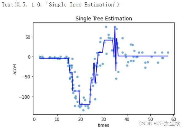

可以看出,单颗决策树的回归线都是矩形,类似楼梯,不平滑,下面进行bagging的方法
Bagging estimation
model = BaggingRegressor(base_estimator=DecisionTreeRegressor(random_state=123), n_estimators=500, random_state=0)
pred_bag = model.fit(X, y).predict(X)
print(model.score(X,y))
sns.scatterplot(x='times', y='accel', data=mcycle, alpha=0.6)
plt.plot(X, pred_bag, 'b')
plt.title('Bagging Estimation')

Alternatively,one could use 'RandomForestRegressor', which by default
sets max_features = n_features that is de facto bagging. The results are slightly different.

The advantage of 'BaggingRegressor' is the option to use different base learners.
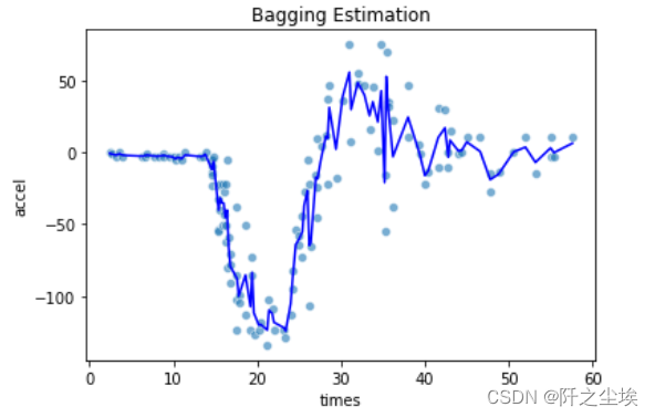
拟合的曲线要平滑很多。
对于回归问题依旧采用最多的波士顿房价数据集,上面依旧导入了包,下面读取数据,划分训练测试集,然后使用bagging拟合:
Boston = load_boston()
X = pd.DataFrame(Boston.data, columns=Boston.feature_names)
y = Boston.target
X_train, X_test, y_train, y_test = train_test_split(X, y, test_size=0.3, random_state=1)

#bagging估计器
model = BaggingRegressor(base_estimator=DecisionTreeRegressor(random_state=123), n_estimators=500, oob_score=True, random_state=0)
#拟合
model.fit(X_train, y_train)
#袋外预测值
pred_oob = model.oob_prediction_
#袋外均方误差
mean_squared_error(y_train, pred_oob)
#袋外测试集拟合优度
model.oob_score_
#测试集拟合优度
model.score(X_test, y_test)
#对比线性回归拟合优度
Comparison with OLS
model = LinearRegression().fit(X_train, y_train)
model.score(X_test, y_test)
观察袋外误差随着估计器的个数变化的图:
OOB Errors

oob_errors = []
for n_estimators in range(100,301,10):
    model = BaggingRegressor(base_estimator=DecisionTreeRegressor(random_state=123),
                          n_estimators=n_estimators, n_jobs=-1, oob_score=True, random_state=0)
    model.fit(X_train, y_train)
    pred_oob = model.oob_prediction_
    oob_errors.append(mean_squared_error(y_train, pred_oob))

plt.plot(range(100, 301,10), oob_errors)
plt.xlabel('Number of Trees')
plt.ylabel('OOB MSE')
plt.title('Bagging OOB Errors')
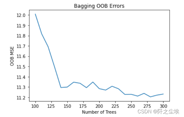
可以看出估计器个数越多,袋外误差越小。
回归森林的Python案例
依旧采用波士顿房价数据集:
Random Forest for Regression on Boston Housing Data
#确定超参数max_features,即每次分裂使用的特征个数
max_features=int(X_train.shape[1] / 3)
max_features
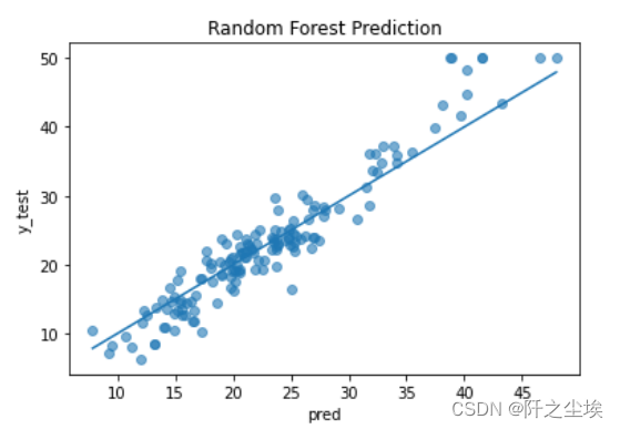
拟合评价
model = RandomForestRegressor(n_estimators=5000, max_features=max_features, random_state=0)
model.fit(X_train, y_train)
model.score(X_test, y_test)
#预测值和真实值比较
Visualize prediction fit
pred = model.predict(X_test)
plt.scatter(pred, y_test, alpha=0.6)
w = np.linspace(min(pred), max(pred), 100)
plt.plot(w, w)
plt.xlabel('pred')
plt.ylabel('y_test')
plt.title('Random Forest Prediction')
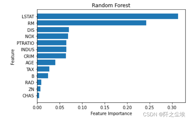
变量重要性的可视化
Feature Importance Plot
model.feature_importances_
sorted_index = model.feature_importances_.argsort()

plt.barh(range(X.shape[1]), model.feature_importances_[sorted_index])
plt.yticks(np.arange(X.shape[1]), X.columns[sorted_index])
plt.xlabel('Feature Importance')
plt.ylabel('Feature')
plt.title('Random Forest')
plt.tight_layout()
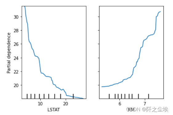
画偏依赖图
from sklearn.inspection import PartialDependenceDisplay
PartialDependenceDisplay.from_estimator(model, X, ['LSTAT', 'RM'])
手工循环,找最优超参数
scores = []
for max_features in range(1, X.shape[1] + 1):
    model = RandomForestRegressor(max_features=max_features,
                                  n_estimators=500, random_state=123)
    model.fit(X_train, y_train)
    score = model.score(X_test, y_test)
    scores.append(score)

index = np.argmax(scores)
range(1, X.shape[1] + 1)[index]

plt.plot(range(1, X.shape[1] + 1), scores, 'o-')
plt.axvline(range(1, X.shape[1] + 1)[index], linestyle='--', color='k', linewidth=1)
plt.xlabel('max_features')
plt.ylabel('R2')
plt.title('Choose max_features via Test Set')
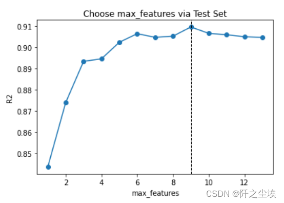
可以看出当max_feature=9时,测试集的拟合优度最高。
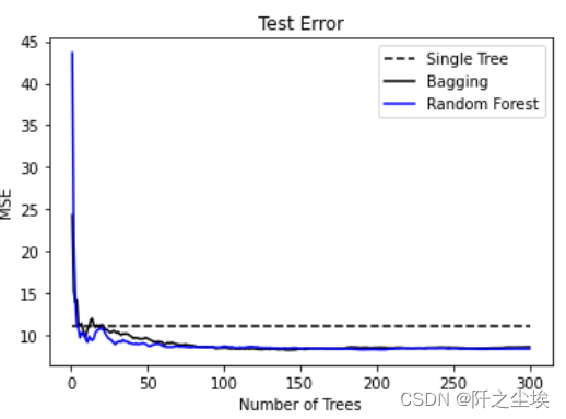
下面比较随机森林,bagging,决策树他们的误差和估计器个数的变化
#RF
scores_rf = []
for n_estimators in range(1, 301):
    model = RandomForestRegressor(max_features=9,
                                  n_estimators=n_estimators, random_state=123)
    model.fit(X_train, y_train)
    pred = model.predict(X_test)
    mse = mean_squared_error(y_test, pred)
    scores_rf.append(mse)

Bagging
scores_bag = []
for n_estimators in range(1, 301):
    model = BaggingRegressor(base_estimator=DecisionTreeRegressor(random_state=123), n_estimators=n_estimators, random_state=0)
    model.fit(X_train, y_train)
    pred = model.predict(X_test)
    mse = mean_squared_error(y_test, pred)
    scores_bag.append(mse)

#DecisionTree
model = DecisionTreeRegressor()
path = model.cost_complexity_pruning_path(X_train, y_train)
param_grid = {'ccp_alpha': path.ccp_alphas}
kfold = KFold(n_splits=10, shuffle=True, random_state=1)
model = GridSearchCV(DecisionTreeRegressor(random_state=123), param_grid, cv=kfold, scoring='neg_mean_squared_error')
model.fit(X_train, y_train)
score_tree = -model.score(X_test, y_test)
scores_tree = [score_tree for i in range(1, 301)]

#画图
plt.plot(range(1, 301), scores_tree, 'k--', label='Single Tree')
plt.plot(range(1, 301), scores_bag, 'k-', label='Bagging')
plt.plot(range(1, 301), scores_rf, 'b-', label='Random Forest')
plt.xlabel('Number of Trees')
plt.ylabel('MSE')
plt.title('Test Error')
plt.legend()
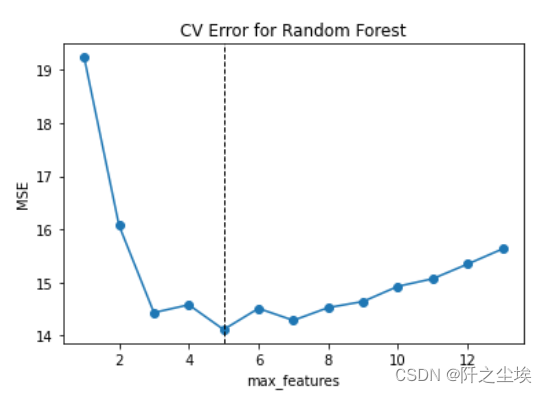
网格化搜索最优超参数
max_features = range(1, X.shape[1] + 1)
param_grid = {'max_features': max_features }
kfold = KFold(n_splits=10, shuffle=True, random_state=1)
model = GridSearchCV(RandomForestRegressor(n_estimators=300, random_state=123),
                     param_grid, cv=kfold, scoring='neg_mean_squared_error', return_train_score=True)

model.fit(X_train, y_train)

model.best_params_

cv_mse = -model.cv_results_['mean_test_score']

plt.plot(max_features, cv_mse, 'o-')
plt.axvline(max_features[np.argmin(cv_mse)], linestyle='--', color='k', linewidth=1)
plt.xlabel('max_features')
plt.ylabel('MSE')
plt.title('CV Error for Random Forest')
分类森林的Python案例
#读取数据
Sonar = pd.read_csv('Sonar.csv')
Sonar.shape
Sonar.head(2)
#取出X和y
X = Sonar.iloc[:, :-1]
y = Sonar.iloc[:, -1]
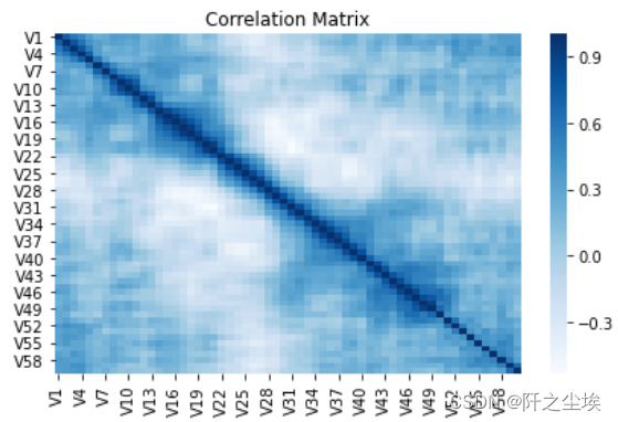
#画变量之间的相关性热力图
sns.heatmap(X.corr(), cmap='Blues')
plt.title('Correlation Matrix')
plt.tight_layout()
划分测试训练集,用决策树和随机森林去拟合比较
X_train, X_test, y_train, y_test = train_test_split(X, y, stratify=y, test_size=50, random_state=1)

Single Tree  as benchmark
model = DecisionTreeClassifier()
path = model.cost_complexity_pruning_path(X_train, y_train)
param_grid = {'ccp_alpha': path.ccp_alphas}
kfold = KFold(n_splits=10, shuffle=True, random_state=1)
model = GridSearchCV(DecisionTreeClassifier(random_state=123), param_grid, cv=kfold)
model.fit(X_train, y_train)
model.score(X_test, y_test)

Random Forest
model = RandomForestClassifier(n_estimators=500, max_features='sqrt', random_state=123)
model.fit(X_train, y_train)
model.score(X_test, y_test)
网格化搜参
Choose optimal mtry parameter via CV
#GridSearchCV需要响应变量y是数值,所以生成虚拟变量
y_train_dummy = pd.get_dummies(y_train)
y_train_dummy = y_train_dummy.iloc[:, 1]
param_grid = {'max_features': range(1, 11) }
kfold = StratifiedKFold(n_splits=10,shuffle=True,random_state=1)
model = GridSearchCV(RandomForestClassifier(n_estimators=300, random_state=123), param_grid, cv=kfold)
model.fit(X_train, y_train_dummy)
model.best_params_
#max_features=8
#因此采用8进行估计
model = RandomForestClassifier(n_estimators=500, max_features=8, random_state=123)
model.fit(X_train, y_train)
model.score(X_test, y_test)
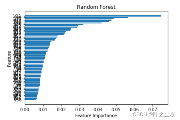
#变量重要性的图
sorted_index = model.feature_importances_.argsort()
plt.barh(range(X.shape[1]), model.feature_importances_[sorted_index])
plt.yticks(np.arange(X.shape[1]), X.columns[sorted_index])
plt.xlabel('Feature Importance')
plt.ylabel('Feature')
plt.title('Random Forest')
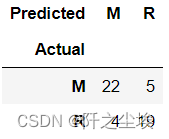
计算混淆矩阵
Prediction Performance
pred = model.predict(X_test)
table = pd.crosstab(y_test, pred, rownames=['Actual'], colnames=['Predicted'])
table
计算混淆矩阵指标
table = np.array(table)
Accuracy = (table[0, 0] + table[1, 1]) / np.sum(table)
Accuracy
Sensitivity = table[1 , 1] / (table[1, 0] + table[1, 1])
Sensitivity
Specificity = table[0, 0] / (table[0, 0] + table[0, 1])
Specificity
Recall = table[1, 1] / (table[0, 1] + table[1, 1])
Recall
cohen_kappa_score(y_test, pred)
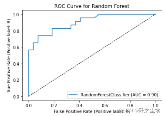
#画ROC曲线
plot_roc_curve(model, X_test, y_test)
x = np.linspace(0, 1, 100)
plt.plot(x, x, 'k--', linewidth=1)
plt.title('ROC Curve for Random Forest')
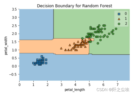
用鸢尾花两个特征变量画其决策边界
X,y = load_iris(return_X_y=True)
X2 = X[:, 2:4]

model = RandomForestClassifier(n_estimators=500, max_features=1, random_state=1)
model.fit(X2,y)
model.score(X2,y)

plot_decision_regions(X2, y, model)
plt.xlabel('petal_length')
plt.ylabel('petal_width')
plt.title('Decision Boundary for Random Forest')
Original: https://blog.csdn.net/weixin_46277779/article/details/125477184
Author: 阡之尘埃
Title: Python机器学习09——随机森林
原创文章受到原创版权保护。转载请注明出处:https://www.johngo689.com/613928/
转载文章受原作者版权保护。转载请注明原作者出处!