MachineLearning 3. 聚类分析（Cluster Analysis）

点击关注，桓峰基因

; 前 言

聚类分析(Cluster Analysis）又称群分析，是根据”物以类聚”的道理，对样品或指标进行分类的一种多元统计分析方法，它们讨论的对象是大量的样品，要求能合理地按各自的特性来进行合理的分类，没有任何模式可供参考或依循，即是在没有先验知识的情况下进行的。聚类分析起源于分类学，在古老的分类学中，人们主要依靠经验和专业知识来实现分类，很少利用数学工具进行定量的分类。随着人类科学技术的发展，对分类的要求越来越高，以致有时仅凭经验和专业知识难以确切地进行分类，于是人们逐渐地把数学工具引用到了分类学中，形成了数值分类学,之后又将多元分析的技术引入到数值分类学形成了聚类分析。

聚类分析的计算方法

[TencentCloudSDKException] code:FailedOperation.ServiceIsolate message:service is stopped due to arrears, please recharge your account in Tencent Cloud requestId:d2c37e18-3d9e-48ed-9d81-f2f92c26a50f

[TencentCloudSDKException] code:FailedOperation.ServiceIsolate message:service is stopped due to arrears, please recharge your account in Tencent Cloud requestId:6621e88f-4a38-40f6-b446-96917efab4cb

1. 分裂法(partitioning methods)；
2. 层次法(hierarchical methods);
3. 基于密度的方法(density-based methods);
4. 基于网格的方法(grid-based methods)；
5. 基于模型的方法(model-based methods)。
6. 分裂法又称划分方法(PAM:PArtitoning methods)首先创建k个划分，k为要创建的划分个数;然后利用一个循环定位技术通过将对象从一个划分移到另一个划分来帮助改善划分质量。典型的划分方法包括:

a.k-means,k-medoids,CLARA(Clustering LARge Application);

b.CLARANS(Clustering Large Application based upon RANdomized Search);

c.FCM.

1. 层次法(hierarchical method)创建一个层次以分解给定的数据集。该方法可以分为自上而下(分解)和自下上(台并)两种操作方式。为弥补分解与合并的不足，层次合并经常要与其它聚类方法相结合，如循环定位。典型的这类方法包括:

a. BRCH(Balanced lterative Reduing and Clustering using Hierarchies)方法，它首先利用树的结构对对象集进行划分;然后再利用其它聚类方法对这些聚类进行优化;

b. CURE(Clustering Using REprisentatives)方法，它利用固定数目代表对象来表示相应聚类;然后对各聚类按照指定量(向聚类中心)进行收缩;

c. ROCK方法，它利用聚类间的连接进行聚类合并;

d. CHEMALOEN方法，它则是在层次聚类时构造动态模型;

1. 基于密度的方法，根据密度完成对象的聚类。它根据对象周围的密度〈如DBSCAN)不断增长聚类。典型的基于密度方法包括:

a. DBSCAN(Densit-based Spatial Clustering of Application with Noise;该算法通过不断生长足够高密度区域来进行聚类;它能从含有噪声的空间数)据库中发现任意形状的聚类。此方法将一个聚类定义为一组”密度连接”的点集; b. OPTICS(Ordering Points To ldentify the Clustering Structure;并不明确产生一个聚类，而是为自动交互的聚类分析计算出一个增强聚类I顺序。

4、基于网格的方法，首先将对象空间划分为有限个单元以构成网格结构;然后利用网格结构完成聚类。典型的基于网格的方法包括:

a. STING(STatistical INformation Grid)就是一个利用网格单元保存的统计信息进行基于网格聚类的方法;

b. CLIQUE(Clustering lIn QUEst)和Wave-Cluster则是一个将基于网格与基于密度相结合的方法。

5、基于模型的方法，它假设每个聚类的模型并发现适合相应模型的数据。

聚类的步骤

(1)选择合适的变量。第一步是选择你感觉可能对识别和理解数据中不同观测值分组有重要影响的变量；

(2)缩放数据。如果我们在分析中选择的变量变化范围很大，那么该变量对结果的影响也是最大的。这往往是不可取的，分析师往往在分析之前缩放数据。最常用的方法有三种：

1.将每个变量标准化为均值为0和标准差为1的变量；

2.每个变量被其最大值相除；

3.该变量减去它的平均值并除以变量的平均绝对偏差。

(3)寻找异常值。许多聚类方法对于异常值是十分敏感的，它能扭曲我们得到的聚类方案。通过outliers包中的函数来筛选（和删除)异常单变量离群点。mvoutlier包中包含了能识别多元变量的离群点的函数。一个替代的方法是使用对异常值稳健的聚类方法，围绕中心点的划分可以很好地解释这种方法；

(4)计算距离。尽管不同的聚类算法差异很大，但是它们通常需要计算被聚类的实体之间的距离。两个观测值之间最常用的距离量度是欧几里得距离，其他可选的量度包括曼哈顿距离、兰氏距离、非对称二元距离、最大距离和闵可夫斯基距离；

(5)选择聚类算法。层次聚类对于小样本来说很实用(如150个观测值或更少),而且这种情况下嵌套聚类更实用。划分的方法能处理更大的数据量，但是需要事先确定聚类的个数。一旦选定层次方法或划分方法，就必须选择一个特定的聚类算法。再次强调每个算法都有优点和缺点。可以尝试多种算法来看看相应结果的稳健性；

(6)获得一种或多种聚类方法。这一步可以使用步骤(5)选择的方法；

(7)确定类的数目。为了得到最终的聚类方案，你必须确定类的数目。对此研究者们也提出了很多相应的解决方法；

(8)获得最终聚类方案。一旦类的个数确定下来，就可以提取出子群，形成最终的聚类方案；

(9)结果可视化。可视化可以帮助你判定聚类方案的意义和用处。层次聚类的结果通常表示为一个树状图。划分的结果通常利用可视化双变量聚类图来表示；

(10)解读类。一旦聚类方案确定，你必须解释这个类。一个类中的观测值有何相似之处?不同的类之间的观测值有何不同?这一步通常通过获得类中每个变量的汇总统计来完成。对于连续数据，每一类中变量的均值和中位数会被计算出来。对于混合数据（数据中包含分类变量),结果中将返回各类的众数或类别分布；

(11)验证结果。验证聚类方案相当于问:”这种划分并不是因为数据集或聚类方法的某种特性，而是确实给出了一个某种程度上有实际意义的结果吗?”如果采用不同的聚类方法或不同的样本，是否会产生相同的类?fpc、clv和clValid包包含了评估聚类解的稳定性的函数。

实例解析

我们这次通过一样的数据分别选择多种方法进行聚类，评估哪种聚类方法更适合RPKM的聚类方法。

1.软件安装

我们选择了5种聚类方法，所以安装的软件包会多一些，如下：

if (!require(flexclust)) {
    install.packages("flexclust")
}
if (!require(NbClust)) {
    install.packages("NbClust")
}
if (!require(cluster)) {
    install.packages("cluster")
}
if (!require(fMultivar)) {
    install.packages("fMultivar")
}
if (!require(Hmisc)) {
    install.packages("Hmisc")
}
if (!require(ggplot2)) {
    install.packages("ggplot2")
}
if (!require(mclust)) {
    install.packages("mclust")
}
if (!require(fpc)) {
    install.packages("fpc")
}
if (!require(optpart)) {
    install.packages("optpart")
}
if (!require(factoextra)) {
    install.packages("factoextra")
}
library(flexclust)
library(NbClust)
library(cluster)
library(fMultivar)
library(Hmisc)
library(ggplot2)
library(mclust)
library(fpc)
library(factoextra)
library(optpart)

2.数据读取

[TencentCloudSDKException] code:FailedOperation.ServiceIsolate message:service is stopped due to arrears, please recharge your account in Tencent Cloud requestId:ceb95c2e-18a3-4151-a841-f4f7dc7f58a7

数据读取
DEG = read.table("DEG-resdata.xls", sep = "\t", check.names = F, header = T)
table(DEG$sig)
##
## Down   Up
## 1296 2832
group <- 1 2 41 478 1351 1735 read.table("deg-group.xls", sep="\t" , check.names="F," header="T)" table(group$group) ## nt tp len <- read.table("all_hg19gene_len.txt", head(len, 2) gene length ddx11l1 wash7p < code></->

我们获得的基因是ENSEMBL，我们需要将其转为SYMOL，如下：

library(org.Hs.eg.db)
library(clusterProfiler)
geneList <- 1 2 3 4 5 6 7123 8029 130749 200931 266675 284723 deg$row.names eg <- bitr(genelist, fromtype="ENSEMBL" , totype="c("ENTREZID"," "ensembl", "symbol"), orgdb="org.Hs.eg.db" ) head(eg) ## ensembl entrezid symbol ensg00000142959 best4 ensg00000163815 clec3b ensg00000107611 cubn ensg00000162461 slc25a34 ensg00000163959 slc51a ensg00000144410 cpo mergedata merge(eg, deg, by.y="Row.names" by.x="ENSEMBL" < code></->

由于我们之前保留的是Count Reads ，所以我们需要将其转为RPKM，转化规则可以看下我们的公众号内容：RNA 12. SCI 文章中肿瘤免疫浸润计算方法之 CIBERSORT RNA 8. SCI文章中差异基因表达–热图 (heatmap)

exp <- 1000 merge(mergedata, len, by.x="SYMBOL" , by.y="Gene" ) exp <- exp[!duplicated(exp$symbol), ] kb exp$length countdata exp[, 10:ncol(exp)] rpk expmat t(t(rpk) colsums(countdata) * 10^6) rownames(expmat)="exp$SYMBOL" expmat[1:3, 1:3] ## tcga-3l-aa1b-01a-11r-a37k-07 tcga-4n-a93t-01a-11r-a37k-07 a2ml1 0.3428737 0.1904078 aacsp1 0.1481661 0.0000000 aadac 4.5036087 3.7514781 tcga-4t-aa8h-01a-11r-a41b-07 9.9516816 0.2905691 1.1776060 < code></->

[TencentCloudSDKException] code:FailedOperation.ServiceIsolate message:service is stopped due to arrears, please recharge your account in Tencent Cloud requestId:433ae636-5c43-4acd-9a19-46abf2a5cc75

set.seed(1234)
sam <- 50 100 2534 sample(ncol(expmat), 100, replace="FALSE)" expmat="expMat[," sam] dim(expmat) ## [1] library(dplyr) set.seed(1234) exp_sample <- sample_n(expmat, 50, # exp_sample<-na.omit(exp_sample) t(exp_sample) dim(exp_sample) exp_sample[1:3, 1:3] il17f f7 ighv3-7 tcga-az-4614-01a-01r-1410-07 1.5826763 192.233246 0.00000 tcga-aa-3524-01a-02r-0821-07 0.0000000 40.575613 tcga-dm-a1d9-01a-11r-a155-07 0.5863731 1.813507 11.64019 < code></->

不同的聚类方法

1.层次聚类

1. hclust {stats}

用一般方法，非常常用的hclust来做，方法有如下几种：

1. euclidean；
2. maximum；
3. manhattan；
4. canberra”；
5. binary；
6. minkowski.

[TencentCloudSDKException] code:FailedOperation.ServiceIsolate message:service is stopped due to arrears, please recharge your account in Tencent Cloud requestId:5418f31f-b701-48ca-ab0e-178789a46c6c

1. ward.D;
2. ward.D2;
3. single;
4. complete;
5. average (= UPGMA);
6. mcquitty (= WPGMA);
7. median (= WPGMC);
8. centroid (= UPGMC).

[TencentCloudSDKException] code:FailedOperation.ServiceIsolate message:service is stopped due to arrears, please recharge your account in Tencent Cloud requestId:2de5aefa-8d03-4fdc-a7dc-4f7ed8a9255a

##########
pdf("cluster.pdf", h = 96, w = 12)
par(mfrow = c(24, 2))
dis = c("euclidean", "maximum", "manhattan", "canberra", "binary", "minkowski")
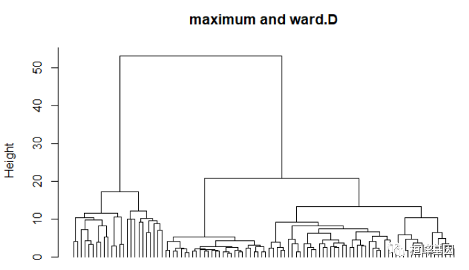
meds <- 2 c("ward.d", "ward.d2", "single", "complete", "average", "mcquitty", "median", "centroid") nom <- scale(exp_sample) for (i in1:length(dis)) { (j in1:length(meds)) d dist(nom, method="dis[i])" hc hclust(d, plot(hc, hang="-1," cex="0.8," main="paste(dis[i]," meds[j], sep=" and " ), labels="FALSE," xlab , sub ) } dev.off() ## png < code></->

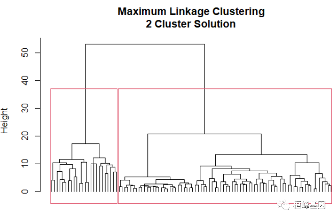
下面的结果看出聚类结果较好的组合是maximum and ward.D或maximum and ward.D2，那么我们就选第一下后面的，如下：

nom <- scale(exp_sample) d <- dist(nom, method="maximum" ) hc hclust(d, plot(hc, hang="-1," cex="0.8," main="maximum and ward.D" , labels="FALSE," xlab sub < code></->

2. NbClust {NbClust}

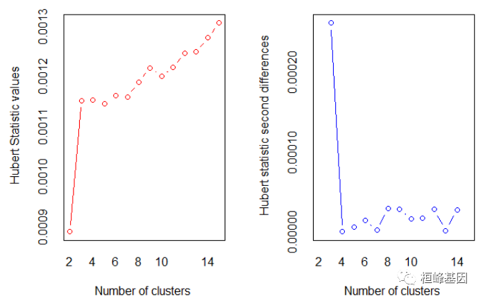
常用方法是尝试不同的类数（比如2～K)并比较解的质量。在NbClust包中的NbClust()函数提供了30个不同的指标来帮助你进行选择。R语言提供了丰富的层次聚类函数，这里我给大家简单介绍一下用Ward方法进行的层次聚类分析。选择聚类的个数，如下：

nc <- nbclust(nom, distance="maximum" , min.nc="2," max.nc="15," method="ward.D" ) < code></->

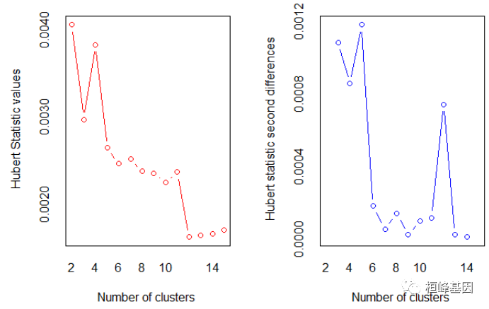
## *** : The Hubert index is a graphical method of determining the number of clusters.

##                 In the plot of Hubert index, we seek a significant knee that corresponds to a
##                 significant increase of the value of the measure i.e the significant peak in Hubert
##                 index second differences plot.

##

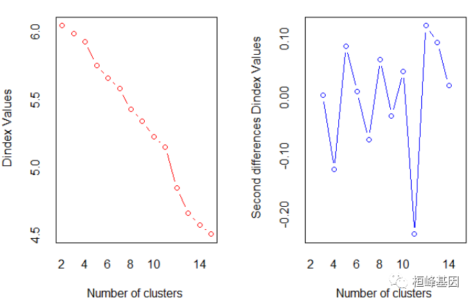
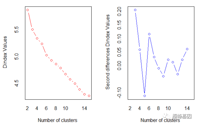
## *** : The D index is a graphical method of determining the number of clusters.

##                 In the plot of D index, we seek a significant knee (the significant peak in Dindex
##                 second differences plot) that corresponds to a significant increase of the value of
##                 the measure.

##
## *******************************************************************
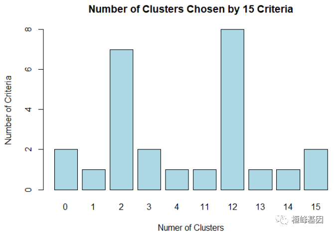
## * Among all indices:
## * 7 proposed 2 as the best number of clusters
## * 2 proposed 3 as the best number of clusters
## * 1 proposed 4 as the best number of clusters
## * 1 proposed 11 as the best number of clusters
## * 8 proposed 12 as the best number of clusters
## * 1 proposed 13 as the best number of clusters
## * 1 proposed 14 as the best number of clusters
## * 2 proposed 15 as the best number of clusters
##
##                    ***** Conclusion *****
##
## * According to the majority rule, the best number of clusters is  12
##
##
## *******************************************************************
table(nc$Best.n[1, ])
##
##  0  1  2  3  4 11 12 13 14 15
##  2  1  7  2  1  1  8  1  1  2

barplot(table(nc$Best.n[1, ]), xlab = "Numer of Clusters", ylab = "Number of Criteria",
    main = "Number of Clusters Chosen by 15 Criteria", col = "lightblue")

[TencentCloudSDKException] code:FailedOperation.ServiceIsolate message:service is stopped due to arrears, please recharge your account in Tencent Cloud requestId:835da461-8621-4927-bc2c-9deac02f7e22

Listing 16.3 - Obtaining the final cluster solution
clusters <- 0 1 2 24 76 cutree(hc, k="2)" table(clusters) ## clusters aggregate(exp_sample, by="list(cluster" = clusters), median) cluster il17f f7 ighv3-7 cmtm5 smyd1 pdcd4 tmem40 0.5885949 2.816345 7.3784166 0.1689894 0.6187506 513.9769 0.5769721 0.9963804 4.799207 0.5056116 0.0000000 0.4159927 445.8797 1.2995444 krt32 card14 spock3 six1 plpp4 linc01630 linc01433 iglv7-43 11.01663 2.003168 22.92558 0.02081256 2.288693 76.82389 0.1844749 12.39139 2.512881 15.60184 0.00000000 2.534744 104.89287 cyp2d8p fam180b igfbp1 emilin3 mmp3 ky arntl2 inhba 7.468996 0.2696951 1.283745 1.736065 289.3306 0.5925788 84.30983 74.43746 8.259506 2.837076 1.978977 526.1924 0.4384617 75.41280 89.01513 gcg rundc3b ccl8 rna5sp123 cadps alkal2 tmeff2 cd160 1.141907 6.913850 24.13523 3.926224 25.72227 4.281868 0.1002217 2.634259 2.521290 3.643218 17.15406 0.000000 17.71174 6.338635 2.692410 igfbp7-as1 linc01749 edn2 asb11 linc00052 igkv1d-17 snora54 ripply1 0.8244369 0.05529321 10.062267 6.083275 1.960834 7.1290982 0.25768473 8.645022 7.798438 8.620298 1.691099 linc01929 ervv-2 dbndd1 dnase1l3 st8sia3 lgals9c eif3ip1 npy2r 0.8043869 115.6272 8.462869 0.03101895 8.613400 0.4656158 0.7878984 134.7018 11.672475 0.03818862 6.604742 2.6208526 igkv1-17 tacstd2 mir3941 285.7966 139.45623 194.6544 88.77291 aggregate(as.data.frame(nom), -0.2880191 -0.3312677 -0.3516608 -0.2474067 -0.2620227 0.05681396 -0.2312050 -0.3016563 -0.4114248 -0.3324179 -0.2899677 -0.24847137 -0.3355040 -0.2353572 -0.3266249 -0.2581192 -0.3293945 -0.2408573 -0.2658946 -0.1894173 -0.2147371 -0.2394491 -0.2631967 -0.4262673 -0.2873070 -0.3010961 -0.4629829 -0.3139076 -0.2568656 -0.3000304 -0.18644310 -0.2426877 -0.4016761 -0.2428107 -0.3276591 -0.2602157 -0.06684606 -0.30056784 -0.1298538 -0.2745230 -0.2450213 -0.4230769 -0.2710479 -0.3408637 -0.07308097 -0.1805193 -0.3744222 -0.1199038 -0.3879564 -0.5768739 -0.5078703 -0.1504334 -0.2797459 -0.2216113 -0.1749399 -0.1781910 -0.19369512 -0.2327267 -0.1863332 -0.4496976 -0.1055253 -0.2213039 -0.1571879 -0.03549121 -0.1805199 -0.3856065 -0.1625653 -0.1369634 -0.2887597 -0.1818619 -0.3099469 -0.2742967 -0.4653439 -0.2680339 -0.1618842 -0.3403107 -0.2777713 -0.3872932 -0.21988468 -0.4127087 -0.3828443 -0.3413641 -0.4650979 -0.5097886 -0.05964795 -0.3105041 -0.3532432 -0.4200815 -0.2856910 -0.4301185 -0.3442862 -0.4263927 -0.5403581 -0.4053723 plot(hc, hang="-1," cex="0.8," main="Maximum Linkage Clustering\n2 Cluster Solution" , labels="FALSE," sub xlab ) rect.hclust(hc, < code></->

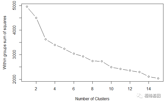
利用碎石图确定聚类个数,如下：

Plot function for within groups sum of squares by number of clusters
wssplot <- function(data, nc="15," seed="1234)" { wss <- (nrow(data) - 1) * sum(apply(data, 2, var)) for (i in2:nc) set.seed(seed) wss[i] sum(kmeans(data, centers="i)$withinss)" } plot(1:nc, wss, type="b" , xlab="Number of Clusters" ylab="Within groups sum of squares" ) wssplot(nom) < code></->

3. K-means

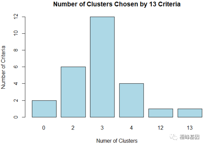
在聚类分析中，K-means聚类算法是最常用的，它需要分析者先确定要将这组数据分成多少类，也即聚类的个数，这个通常可以用因子分析的方法来确定。比如我们可以用”nFactors”包的函数来确定最佳的因子个数，将因子数作为聚类数，不过关于聚类个数的确定还要考虑数据的实际情况与自身需求，这样分析才会更具有现实意义。另外，我们也可以通过绘制碎石图来确定聚类个数，这和主成分的思想相似。

set.seed(1234)
nc <- nbclust(nom, min.nc="2," max.nc="15," method="kmeans" ) < code></->

## *** : The Hubert index is a graphical method of determining the number of clusters.

##                 In the plot of Hubert index, we seek a significant knee that corresponds to a
##                 significant increase of the value of the measure i.e the significant peak in Hubert
##                 index second differences plot.

##

## *** : The D index is a graphical method of determining the number of clusters.

##                 In the plot of D index, we seek a significant knee (the significant peak in Dindex
##                 second differences plot) that corresponds to a significant increase of the value of
##                 the measure.

##
## *******************************************************************
## * Among all indices:
## * 6 proposed 2 as the best number of clusters
## * 12 proposed 3 as the best number of clusters
## * 4 proposed 4 as the best number of clusters
## * 1 proposed 12 as the best number of clusters
## * 1 proposed 13 as the best number of clusters
##
##                    ***** Conclusion *****
##
## * According to the majority rule, the best number of clusters is  3
##
##
## *******************************************************************
table(nc$Best.n[1, ])  # 决定聚类个数
##
##  0  2  3  4 12 13
##  2  6 12  4  1  1

[TencentCloudSDKException] code:FailedOperation.ServiceIsolate message:service is stopped due to arrears, please recharge your account in Tencent Cloud requestId:a13e9f6f-82fe-4bfb-bc17-45f358797b6c

barplot(table(nc$Best.n[1, ]), xlab = "Numer of Clusters", ylab = "Number of Criteria",
    main = "Number of Clusters Chosen by 13 Criteria", col = "lightblue")

进行K均值聚类分析，绘制聚类图，如下：

set.seed(1234)
fit.km <- 1 2 3 11 88 kmeans(nom, 3, nstart="25)" # 进行k均值聚类分析 head(fit.km$size) ## [1] head(fit.km$centers) il17f f7 ighv3-7 cmtm5 smyd1 pdcd4 -0.3033558 -0.26190722 1.4055743 0.4082672 0.2498796 0.69684023 0.0421243 0.02517585 -0.1709715 -0.1522383 -0.1231630 -0.08641151 -0.3700242 0.66550478 -0.4158215 8.9060298 8.0896682 -0.06102960 tmem40 krt32 card14 spock3 six1 plpp4 -0.362363108 -0.22065253 -0.78214969 0.11952882 -0.55062557 -0.7788310 0.005027673 -0.00806648 0.07851735 -0.04062087 0.07074427 0.1038498 3.543558958 3.13702805 1.69412011 2.25981933 -0.16861467 -0.5716388 linc01630 linc01433 iglv7-43 cyp2d8p fam180b igfbp1 -0.24579463 -0.65201479 1.2035853 -0.68438367 0.7997951 -0.31833860 -0.05810688 0.02298383 -0.1466840 0.02431761 -0.1718955 0.03427224 7.81714632 5.14958598 -0.3312469 5.38827060 6.3290583 0.48576776 emilin3 mmp3 ky arntl2 inhba gcg 0.8095011 -0.46443987 -0.14329723 -0.8842087 -0.79163943 2.26939837 -0.1671745 0.05721899 -0.09203014 0.1189363 0.09411268 -0.28280319 5.8068424 0.07356759 9.67492155 -0.7400995 0.42611749 -0.07670164 rundc3b ccl8 rna5sp123 cadps alkal2 tmeff2 0.45673682 0.41538110 -0.130832591 -0.568783015 0.269797780 0.2654644 -0.07048812 -0.05666444 0.003104592 0.071202484 -0.033612042 -0.1422725 1.17884953 0.41727843 1.165954384 -0.009205451 -0.009915867 9.5998700 cd160 igfbp7-as1 linc01749 edn2 asb11 linc00052 -0.03071948 -0.15939844 -0.2331126 0.36867201 -0.07035151 -0.12921182 -0.07427513 0.01659261 -0.0598016 -0.06959498 -0.10312412 -0.09439828 6.87412605 0.29323277 7.8267799 2.06896647 9.84878886 9.72837895 igkv1d-17 snora54 ripply1 linc01929 ervv-2 dbndd1 1.1706605 -0.16585298 -0.47669118 -0.30734680 -0.27433892 -0.8699670 -0.1603865 0.02279823 -0.02897558 0.04346155 0.03869342 0.1093077 1.2367475 -0.18186187 7.79345442 -0.44380136 -0.38729319 -0.0494384 dnase1l3 st8sia3 lgals9c eif3ip1 npy2r igkv1-17 1.7339587 0.5752728 0.9766528 -0.35904218 2.2800690 0.75062759 -0.2231538 -0.1345245 -0.1423932 0.05060592 -0.2792156 -0.08565249 0.5639854 5.5101569 1.7874242 -0.50385688 -0.5097886 -0.71948427 tacstd2 mir3941 -0.49459774 -0.31656432 0.05944485 0.04441591 0.20942843 -0.42639268 aggregate(exp_sample, by="list(cluster" = fit.km$cluster), mean) cluster 0.4785149 7.460917 209.45886 1.4723694 4.332919 656.7416 0.444122 2.9582112 26.684794 28.15752 0.3581697 1.626264 482.0289 2.261306 0.0000000 69.562991 0.00000 18.3646297 61.215432 487.6906 19.763545 0.1315531 3.833043 1.1778745 0.2997228 1.675485 0.0403494 0.8104104 2.0334175 17.405693 0.6783717 5.0841760 36.541595 0.2227790 3.6539136 30.1704631 42.883618 7.8533855 3.2411486 9.859628 7.8774055 25.2502680 839.8532 3.349757 4.2951477 0.5694678 3.758912 118.7052 0.5516859 221.6396 11.229645 0.5933968 14.3262393 1.775201 661.8622 0.7076329 137.1385 70.870215 25.3594190 31.9409017 13.908933 678.8845 30.4172776 30.01116 10.75001 106.891035 14.697087 55.74761 6.069886 12.09875 119.35135 113.95056 6.651268 9.058721 36.01527 20.718074 42.26393 42.84554 152.63303 14.746072 22.419665 55.82692 147.894427 38.47397 12.988460 1.0522118 3.042562 2.191211 0.05379713 23.46872 0.2065057 7.612765 0.1708365 2.921970 9.204716 0.72567688 15.67902 0.1331140 8.032605 21.2297187 22.159956 20.229238 31.29981141 53.68956 22.4196647 0.01406769 126.8576 6.907777 0.4795657 0.6475473 0.1455193 38.24107 0.07724792 16.7068 88.310073 4.4568368 2.3123139 0.5487996 154.81437 17.90380144 132.3266 0.000000 73.9472135 135.91717 75.87623 0.2630833 42.24571 1.739676 2.6566259 1261.99486 14.74231 0.5053909 14.41560 0.0911642 13.69061 6.660828 0.2195618 570.58862 474.43309 2.1664932 39.13471 1.4583557 62.93446 46.55936 598.87492 < code></->

[TencentCloudSDKException] code:FailedOperation.ServiceIsolate message:service is stopped due to arrears, please recharge your account in Tencent Cloud requestId:f5c72a10-2fc6-4a51-bfed-a85cf4113390

NT <- 0 1 2 3 8 88 group[group$group="=" "nt", ] exp_sample$group="ifelse(rownames(exp_sample)" %in% nt$sample, 1, 2) ct.km <- table(exp_sample$group, fit.km$cluster) ## randindex(ct.km) ari 0.7449018 < code></->

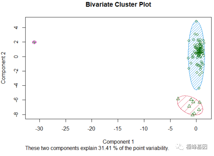
2. 分裂聚类 pam{cluster}

利用PAM（Partitioning around mediods）进行分析，如下：

Listing 16.5 - Partitioning around mediods for the DEG data
set.seed(1234)
fit.pam <- 0 1 2 pam(exp_sample, k="3," stand="TRUE)" head(fit.pam$medoids) ## il17f f7 ighv3-7 cmtm5 tcga-t9-a92h-01a-11r-a37k-07 0.6943772 1.7570762 15.50722 0.7731135 tcga-az-6599-11a-01r-1774-07 0.0000000 0.3429155 104.41179 2.4895665 tcga-cm-4748-01a-01r-1410-07 69.5629914 0.00000 18.3646297 smyd1 pdcd4 tmem40 krt32 card14 533.3114 2.0800125 0.4233717 19.67791 0.6601123 706.5871 0.1217822 2.80102 61.2154324 487.6906 19.7635450 30.1704631 42.88362 spock3 six1 plpp4 linc01630 linc01433 0.000000 0.6822288 6.226054 0.05527045 3.1889546 2.226043 0.2396619 2.187167 0.01618009 0.3111823 7.853385 3.2411486 9.859628 7.87740551 25.2502680 iglv7-43 cyp2d8p fam180b igfbp1 emilin3 21.16858 18.895448 1.067580 0.8964313 1.756613 496.32119 1.164532 3.750329 0.3936371 3.313977 137.13847 70.870215 25.359419 31.9409017 13.908933 mmp3 ky arntl2 inhba 3.617678 0.2561011 125.517002 75.500094 2.753538 0.1124580 9.535511 3.500819 678.884526 30.4172776 42.845543 152.633034 gcg rundc3b ccl8 rna5sp123 cadps 0.9311694 2.674163 1.76265 0.0000 23.130995 127.3923166 12.663665 82.04478 3.719115 14.7460719 22.419665 55.82692 147.8944 38.473970 alkal2 tmeff2 cd160 igfbp7-as1 3.719719 1.679200 16.234881 1.111942 2.621736 0.3739553 8.032605 21.229719 22.159956 20.2292377 linc01749 edn2 asb11 linc00052 igkv1d-17 38.42376 0.4719111 2.78534 0.0551052 28.98096 0.2072236 15.90013 31.2998114 53.68956 22.4196647 17.9038 132.32659 snora54 ripply1 linc01929 ervv-2 dbndd1 12.04716 2.5709479 116.911028 0.5467917 0.2052625 6.609587 73.9472135 135.917170 dnase1l3 st8sia3 lgals9c eif3ip1 npy2r 4.001051 0.1227876 21.97454 0.2042173 33.278217 0.6290431 27.51096 0.4485916 3.8261354 39.134707 1.4583557 62.93446 igkv1-17 tacstd2 mir3941 group 276.36763 180.261614 1770.72762 8.303047 46.55936 598.874924 clusplot(fit.pam, main="Bivariate Cluster Plot" , color="TRUE," shade="TRUE," labels="1," lines="0)" < code></->

[TencentCloudSDKException] code:FailedOperation.ServiceIsolate message:service is stopped due to arrears, please recharge your account in Tencent Cloud requestId:06eb54c9-d877-46b2-8265-2f89643c260c

evaluate clustering
ct.pam <- 0 1 2 3 8 91 table(exp_sample$group, fit.pam$clustering) ct.pam ## randindex(ct.pam) ari 0.9309073 < code></->

3. 基于模型聚类 Mclust{mclust}

基于模型的聚类方法利用极大似然估计法和贝叶斯准则在大量假定的模型中去选择最佳的聚类模型并确定最佳聚类个数。基于参数化有限高斯混合模型的模型聚类。采用基于层次模型的聚类算法初始化EM算法对模型进行估计。然后根据BIC选取最优模型。从下面的结果来看，将总体聚成两类比较合适,如下：

fit.m <- 1 2 3 4 5 96 100 310 mclust(exp_sample) summary(fit.m) ## ---------------------------------------------------- gaussian finite mixture model fitted by em algorithm mclust eei (diagonal, equal volume and shape) with components: log-likelihood n df bic icl -19190.8 -39809.2 clustering table: plot(fit.m, what="classification" ) # 绘图 < code></->

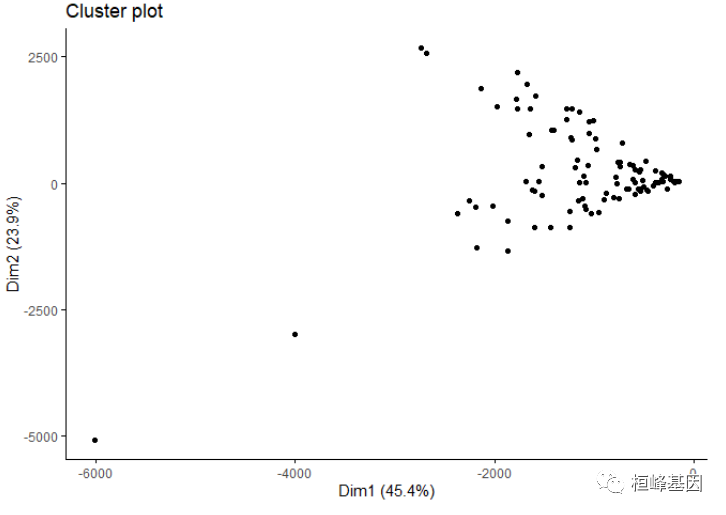
4. 基于密度聚类 dbscan {fpc}

我们介绍一种新的聚类方法，叫DBSCAN（Density-Based Spatial Clustering of Applications with Noise）聚类法，是基于密度的聚类算法,由于差异基因并不适合这种方法聚类，故效果不是很好，如下：

设置随机数种子
set.seed(1234)
db <- dbscan(exp_sample, eps="0.15," minpts="5)" fviz_cluster(db, data="exp_sample," stand="FALSE," ellipse="FALSE," show.clust.cent="FALSE," geom="point" , palette="Set2" ggtheme="theme_classic())" < code></->

[TencentCloudSDKException] code:FailedOperation.ServiceIsolate message:service is stopped due to arrears, please recharge your account in Tencent Cloud requestId:8b3bebe3-d37a-4ac4-95ec-d9102aa8cb0c

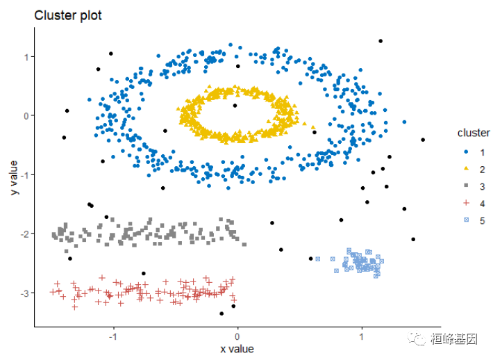
data("multishapes")
df <- multishapes[, 1:2] set.seed(123) db <- dbscan(df, eps="0.15," minpts="5)" fviz_cluster(db, data="df," stand="FALSE," ellipse="FALSE," show.clust.cent="FALSE," geom="point" , palette="jco" ggtheme="theme_classic())" < code></->

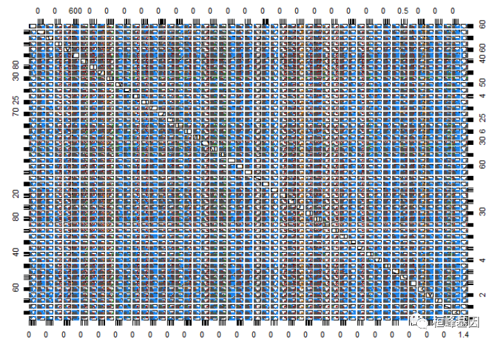
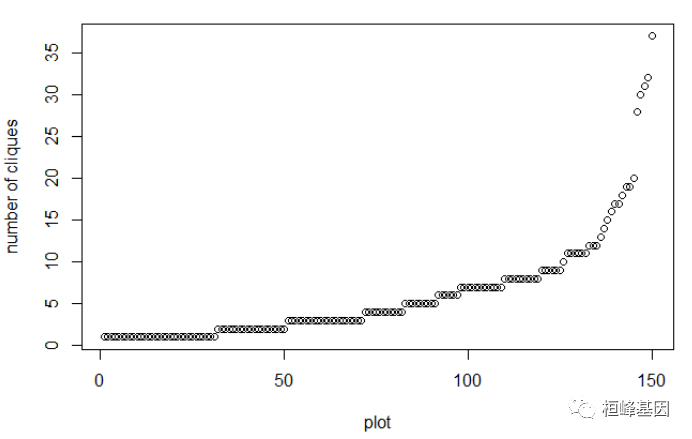
5. 基于网格聚类 clique {optpart}

[TencentCloudSDKException] code:FailedOperation.ServiceIsolate message:service is stopped due to arrears, please recharge your account in Tencent Cloud requestId:4e0e08a2-91a6-4bb3-81e7-766fc6055110

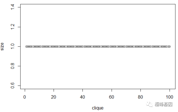
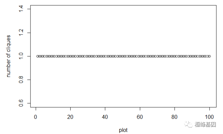
cq <- 100 clique(d, 0.5) summary(cq) ## maximal cliques at alphac="0.5" minimum size="1" maximum plot(cq, panel="all" ) < code></->

## hit return to continue :

[TencentCloudSDKException] code:FailedOperation.ServiceIsolate message:service is stopped due to arrears, please recharge your account in Tencent Cloud requestId:a44e0ff3-919d-4e12-b699-e16d42212529

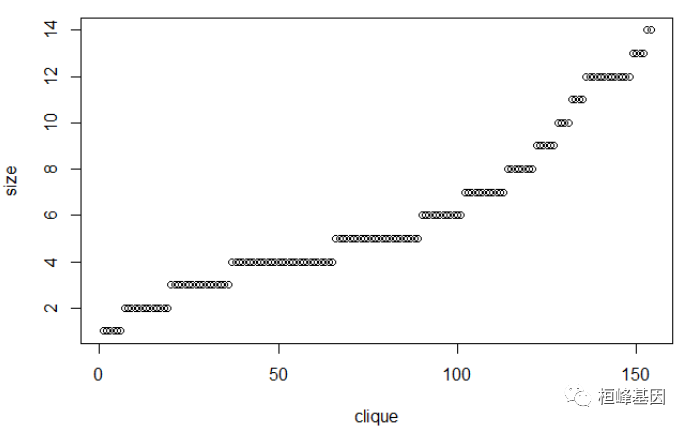
data("iris")
iris2 <- iris[-5] dist.e="dist(iris2," method="euclidean" ) cq <- clique(dist.e, 0.5) # summary(cq) plot(cq) < code></->

## hit return to continue :

结果解读

从五种聚类方法的结果来看，该样本是正常组织和癌组织的差异基因分类，理论上应该是分两类，其中kmeans层次法和分裂法pam的聚类结果较好，评估结果分别是0.74和0.93，所以最后应该选择分裂法对表达差异的样本进行聚类，而基于密度，网格和模型的聚类方法适合比较特殊的数据，目前还没有遇到，不好意思了！

B站直播课，肿瘤克隆进化生信分析培训课程，没有录播，有需要这方面分析内容的老师可以过来交流一下！

[TencentCloudSDKException] code:FailedOperation.ServiceIsolate message:service is stopped due to arrears, please recharge your account in Tencent Cloud requestId:9b505b57-260f-45d7-abf7-fd6c6466cf2f

Topic 1.克隆进化之sciClone
Topic 2.克隆进化之ClonEvol
Topic 3. 克隆进化之 fishplot
Topic 4. 克隆进化之 Pyclone
Topic 5. 克隆进化之 CITUP
Topic 6. 克隆进化之 Canopy
Topic 7. 克隆进化之 Cardelino
Topic 8. 克隆进化之 RobustClone
Topic 9. 克隆进化之 TimeScape
Clone 1. 肿瘤克隆进化之前世今生
Clone 2. 肿瘤克隆进化之不同进化模

[TencentCloudSDKException] code:FailedOperation.ServiceIsolate message:service is stopped due to arrears, please recharge your account in Tencent Cloud requestId:5adfda56-268d-4560-828b-7a996672b91c

; References:

1. Scrucca L., Fop M., Murphy T. B. and Raftery A. E. (2016) mclust 5: clustering, classification and density estimation using Gaussian finite mixture models, The R Journal, 8/1, pp. 289-317.

2. Fraley C. and Raftery A. E. (2002) Model-based clustering, discriminant analysis and density estimation, Journal of the American Statistical Association, 97/458, pp. 611-631.

3. Fraley C., Raftery A. E., Murphy T. B. and Scrucca L. (2012) mclust Version 4 for R: Normal Mixture Modeling for Model-Based Clustering, Classification, and Density Estimation. Technical Report No. 597, Department of Statistics, University of Washington.

4. C. Fraley and A. E. Raftery (2007) Bayesian regularization for normal mixture estimation and model-based clustering. Journal of Classification, 24, 155-18

Original: https://blog.csdn.net/weixin_41368414/article/details/124333227
Author: 桓峰基因
Title: MachineLearning 3. 聚类分析（Cluster Analysis）