

项目名称
动手教你学故障诊断:Python实现基于Tensorflow+CNN深度学习的轴承故障诊断(西储大学数据集)(含完整代码)
项目介绍
该项目使用tensorflow和keras搭建深度学习CNN网络,并使用西储大学数据集作为训练集和测试集,对西储大学mat格式数据进行处理,将数据放入搭建好的网络中进行训练,最终得到相关故障诊断模型。
背景
最近在上故障诊断的课程,老师发给我们西储大学的轴承故障数据集,让我们自己去折腾。正巧前段时间学习了深度学习的课程,因此想着自己搭建一个深度学习的网络来进行相关故障的诊断。查阅相关文献,使用深度学习的故障诊断方法目前主要有两种形式,一种是直接将相关加速度一维数据放入深度学习网络中学习,另一种方式是使用相关变化将加速度数据转为二维图像,将二维图像放入深度学习网络进行学习。本文采用的是第一种方法,接下来对代码相关部分进行介绍,想要学习实践的也可以直接跳到最后有完整代码。
目录
*
– 项目名称
– 项目介绍
–
+ 背景
– 项目相关展示
–
+
* 基本环境介绍
* 数据预处理
* 训练部分
+ 完整源码下载地址
项目相关展示
基本环境介绍
电脑环境:
Windows10
Python环境:
Conda + python3.7
Tensorflow:1.7.1
keras
h5py==2.10.0
数据预处理
下面的代码可以实现数据的预处理,深度学习使用的数据需要我们进行随机划分训练集和测试集,并对相关的数据集打标签。一般我们使用的是0-1编码作为标签,这样做更有利于网络的计算。
from scipy.io import loadmat
import numpy as np
import os
from sklearn import preprocessing
from sklearn.model_selection import StratifiedShuffleSplit
def prepro(d_path, length=864, number=1000, normal=True, rate=[0.5, 0.25, 0.25], enc=True, enc_step=28):
"""对数据进行预处理,返回train_X, train_Y, valid_X, valid_Y, test_X, test_Y样本.
:param d_path: 源数据地址
:param length: 信号长度,默认2个信号周期,864
:param number: 每种信号个数,总共10类,默认每个类别1000个数据
:param normal: 是否标准化.True,False.默认True
:param rate: 训练集/验证集/测试集比例.默认[0.5,0.25,0.25],相加要等于1
:param enc: 训练集、验证集是否采用数据增强.Bool,默认True
:param enc_step: 增强数据集采样顺延间隔
:return: Train_X, Train_Y, Valid_X, Valid_Y, Test_X, Test_Y
import preprocess.preprocess_nonoise as pre
train_X, train_Y, valid_X, valid_Y, test_X, test_Y = pre.prepro(d_path=path,
length=864,
number=1000,
normal=False,
rate=[0.5, 0.25, 0.25],
enc=True,
enc_step=28)
训练部分
数据处理完之后,就是我们的训练部分了,我们首先看一下我的CNN网络架构。
data_input=Input(shape=(4000,1))

conv1=convolutional.Conv1D(128,3,strides=3,padding="same")(data_input)
conv1=BatchNormalization(momentum=0.8)(conv1)
conv1=MaxPool1D(pool_size=4)(conv1)

conv2=convolutional.Conv1D(128,3,strides=3,padding="same")(conv1)
conv2=BatchNormalization(momentum=0.8)(conv2)
conv2=MaxPool1D(pool_size=4)(conv2)

conv3=convolutional.Conv1D(128,3,strides=3,padding="same")(conv2)
conv3=BatchNormalization(momentum=0.8)(conv3)
conv3=MaxPool1D(pool_size=4)(conv3)

flatten=Flatten()(conv3)
dense_1=Dense(128)(flatten)
dense_1=Dropout(0.3)(dense_1)

output = Dense(3, activation='softmax')(dense_1)

cnn_model= Model(input=data_input, output=output)
cnn_model.summary()
上面的部分就是我们的网络架构,就是比较传统的CNN网络架构,如果有不太了解的小伙伴可以留言或者自行查阅相关资料,如果有想了解的朋友比较多,我也可以单独出一篇博客进行详细讲解。
有了网络模型和数据之后我们就可以进行训练了,训练部分代码如下:
def train(cnn_model):

    epoch = 50
    filepath = "model\cnn-"+str(step)+"_weights"+str(epoch)+"-improvement-{epoch:02d}-{val_acc:.2f}.hdf5"

    checkpoint = ModelCheckpoint(filepath, monitor='val_acc', verbose=1, save_best_only=True, mode='max')
    callbacks_list = [checkpoint]

    cnn_model.compile(optimizer=Adam(lr=adam_lr),
                      loss='categorical_crossentropy',metrics=['accuracy'])

    history = cnn_model.fit( X_train, y_train, batch_size=128, epochs=epoch, verbose=1, validation_data=[X_test,y_test],callbacks=callbacks_list)

    epochs = range(epoch)
    plt.figure()
    plt.plot(epochs, history.history['acc'], 'b', label='Training acc')
    plt.plot(epochs, history.history['val_acc'], 'r', label='Validation acc')
    plt.title('Traing and Validation accuracy')
    plt.legend()
    plt.savefig('model_'+str(step)+'_'+str(epoch)+'V0.1_acc.jpg')

    plt.figure()
    plt.plot(epochs, history.history['loss'], 'b', label='Training loss')
    plt.plot(epochs, history.history['val_loss'], 'r', label='Validation val_loss')
    plt.title('Traing and Validation loss')
    plt.legend()
    plt.savefig('model_'+str(step)+'V1'+str(epoch)+'_loss.jpg')
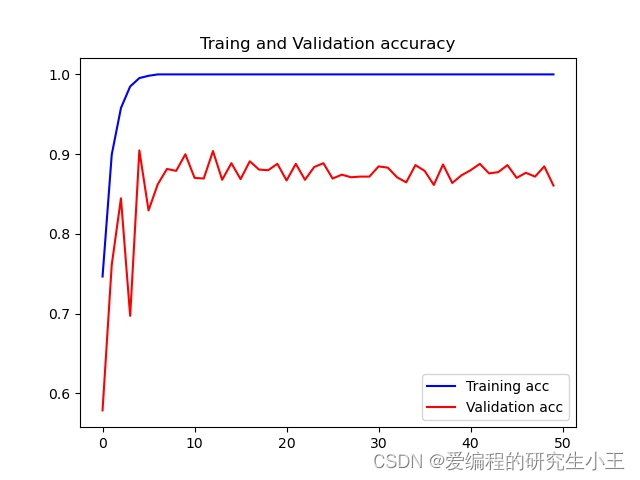
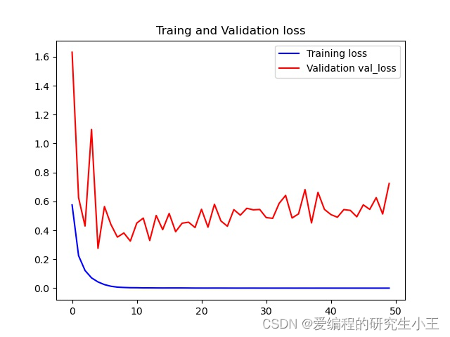
在上面的代码中,我使用了回调函数call_back_list,将该段函数加入后,模型训练中会帮我们保存所有有提升的模型。plot函数可以进行画图,我们可以画出我们训练过程中所有的准确率,损失函数值,得到我们的准确率图像和损失函数。准确率函数图像如下。因为电脑配置有限,因此我只选取了50次作为案例,如果希望图像更好可以尝试更多的次数。

损失函数
完整源码下载地址
基于Python+CNN深度学习的轴承故障诊断 完整代码下载
Original: https://blog.csdn.net/qq_34211771/article/details/125212385
Author: 爱编程的研究生小王
Title: 【动手教你学故障诊断:Python实现Tensorflow+CNN深度学习的轴承故障诊断(西储大学数据集)(含完整代码)】
原创文章受到原创版权保护。转载请注明出处:https://www.johngo689.com/522072/
转载文章受原作者版权保护。转载请注明原作者出处!