

基于卷积神经网络的图像识别技术从入门到深爱(理论与代码实践齐飞!)
- 零、前言
- 一、手写数字识别入门神经网络(入门篇)
* - 1. 手写数字数据集及神经网络数据概念介绍
– - 2. 基于最邻近分类法实现手写数字识别
– - 3. 基于神经网络实现手写数字识别
– - 4. 基于卷积神经网络实现手写数字识别
– - 二、遥感图像分类吃透各种卷积神经网络模型(提升篇)
* - 1. LeNet-5实现遥感图像分类
– - 2. AlexNet实现遥感图像分类
– - 3. VGGNet实现遥感图像分类
– - 4. GoogleNet实现遥感图像分类
– - 5. ResNet实现遥感图像分类
–
零、前言
本文通过手写数字识别作为神经网络理论与代码实践的入门篇,基于入门篇详细讲解各种神经网络的结构及特点并将其应用于遥感图像分类的实践上,所有神经网络代码实现环境为Tensorflow2.0以上。本文总结参考自B站UP主 tm9161,感谢UP主的无私贡献。文章内容表述可能有些不严谨的地方,欢迎评论区留言指正。
如果对机器学习基础感兴趣的,可以移步到我们机器学习专栏,里面机器学习(一)到机器学习(十二)可以作为本篇文章的基础
一、基于神经网络的手写数字识别导论(导论)
[En]
I. introduction to handwritten digit recognition based on Neural Network (introduction)
1. 手写数字数据集及神经网络数据概念介绍
1.1 手写数字数据集
手写数字数据集是由tensorflow官方提供的数据集,可以通过tf.keras.datasets.mnist.load_data()获取训练数据MNIST。MNIST包含70000张手写数字图像:60000张用于训练;10000张用于测试。每张图片是28×28像素的灰度图。


实战代码
(train_images, train_labels), (test_images, test_labels) = tf.keras.datasets.mnist.load_data()
1.2 神经网络数据集
将神经网络数据集细分为训练集、验证集和测试集。例如,对于这三个概念,它很容易理解。神经网络就像一个学生。如果这个学生想要为考试学习知识,他首先需要做很多练习来学习知识。然后根据所学知识做模拟题,验证自己是如何通过练习掌握所学知识的,最终真正拿到试题参考试题。训练集可以理解为练习,验证集可以理解为模拟题,测试集可以理解为试题。
[En]
The neural network data set is subdivided into training set, verification set and test set. For these three concepts, for example, it is easy to understand. The neural network is like a student. If this student wants to learn knowledge for the exam, he needs to do a lot of exercises to learn knowledge first. Then according to the learning knowledge to do simulation questions to verify how he mastered the knowledge learned through practice, and finally really get the examination questions reference exam. The training set can be understood as exercises, the verification set can be understood as simulation questions, and the test set can be understood as examination questions.

至于入学考试,如果他每一道模拟题都做得好,他也可以得出结论,他会在考试中取得好成绩,所以很多神经网络训练都把验证集和测试集归为一类,只剩下训练集和测试集两类。
[En]
As for the entrance examination, if he does well in each simulation question, he can also come to the conclusion that he will get good results in the exam, so many neural network training classifies the verification set and the test set into one category, leaving only two categories: the training set and the test set.

; 1.3 基于tensorflow实现神经神经网络常用的包
import tensorflow as tf

import numpy as np
import pandas as pd

import matplotlib.pyplot as plt
1.4 one-hot编码
对于分类问题,比如被分成三类,我们一般将第一类识别为数字1,第二类识别为数字2,第三分类识别为数字3,但实际上机器可能会错误地认为数字1和2之间有任何关系,例如1和2之间的接近程度,它们之间是否有关系等,所以我们将第一类表示为数字1,第二类表示为数字2,第三类表示为数字3,这类似于二进制形式。所以所有类型的徽标都只由0和1组成。
[En]
For classification problems, such as being divided into three categories, we generally identify the first category as the number 1, the second category as the number 2, and the third category as the number 3. But in fact, it is possible for the machine to mistakenly think that there is any relationship between the number 1 and 2, such as the proximity between 1 and 2, whether there is any relationship between them, and so on, so we will express the first category as the number 1, the second as the number 2, and the third as the number 3, which is similar to the binary form. So that all kinds of logos are only made up of 0 and 1.
如分类为三类的问题中,1转为热编码就是100;2转为热编码就是010;3转为热编码就是001;即第几个位置上的数字为1,那么这个位置就是类别标识。、
pandas包封装了将标识(标签)转为one-hot编码的方法,代码实现如下:
(train_images, train_labels), (test_images, test_labels) = tf.keras.datasets.mnist.load_data()
train_labels = np.array(pd.get_dummies(train_labels))
test_labels = np.array(pd.get_dummies(test_labels))
2. 基于最邻近分类法实现手写数字识别
2.1 最近邻算法原理
对于测试样本,我们计算训练样本集中哪个训练样本最接近哪个训练样本,则测试样本的类别与哪个训练样本的类别相同。也就是说,训练样本集中每个图片的类别是已知的,对于不知道类别的测试样本图片,哪个训练样本图片与训练样本图片的类别接近,则与训练样本图片的类别一致。
[En]
For a test sample, we calculate which training sample is closest to which training sample in the training sample set, then the category of the test sample is the same as that of which training sample. That is, the category of each picture in the training sample set is known, and for a test sample picture that does not know the category, which training sample picture is close to it, it is consistent with the category of the training sample picture.
这里面牵涉到一个 距离的概念。距离的度量有很多种方式,我们常用的有曼哈顿距离和欧氏距离。曼哈顿距离即两点之间所经实际各个路段之和,这也是我们生活中常用的距离概念;而欧式距离是两点之间直接相连的直线距离。下图中红线代表曼哈顿距离,绿线代表欧式距离。

我们使用曼哈顿距离来计算两张图片之间的距离,即两张图片对应位置的像素值之差取绝对值,然后求和。
[En]
We use the Manhattan distance to calculate the distance between the two pictures, that is, the difference between the pixel values of the corresponding positions of the two pictures to take the absolute value, and then summed up.

利用numpy包的api实现代码如下:
np.sum(np.abs(test_data-train_data))
上面代码得到是一个n*1的向量 ,即测试图片距离每张训练图片的距离大小。我们可以找出其中距离最近的那张训练图片,实现代码如下:
train_index = np.argmin(np.sum(np.abs(test_data-train_data),axis=1))
可以找出其中距离最近的那张训练图片后,那张训练图片对应的类别(标签)就是测试图片的类别(标签),因为此时图片的标签是one-hot编码,我们需要将其转为真正的类别数字,根据one-hot编码规则,可以通过以下代码获取测试图片的类别:
ont_hotlable = train_labels[train_index]
predict = np.argmax(ont_hotlable)
2.2 最近邻手写数字识别代码实现
本算法中,训练集60000张图片,测试集10000张图片。具体每个步骤细节已在2.2讲解,在此不再累赘。
import tensorflow as tf

import numpy as np
import pandas as pd

import matplotlib.pyplot as plt

(train_images, train_labels), (test_images, test_labels) = tf.keras.datasets.mnist.load_data()

train_images = train_images.reshape(60000, 28 * 28)
test_images = test_images.reshape(10000, 28 * 28)

train_images = train_images / 255
test_images = test_images / 255

train_labels = np.array(pd.get_dummies(train_labels))
test_labels = np.array(pd.get_dummies(test_labels))

test = 50
acc = 0
for i in range(test):
    test_data = test_images[i]
    train_data = train_images[:20000, :]

    distance = np.argmin(np.sum(np.abs(test_data - train_data), axis=1))
    predict = np.argmax(train_labels[distance])
    real = np.argmax(test_labels[i])
    if predict == real:

        acc += 1

    print("预测:", predict, "真实:", real)

print("准确率:", acc / test)
2.3 算法问题与改进
- 距离不能反应差别
这种计算的明显问题是,使用简单的曼哈顿距离有时不能准确地实现图像分类,例如,下面的图片本来是同一个人,但因为图片的颜色或封面的一小部分会导致像素值的变化,这会导致距离的计算没有意义,导致无法确定同一个人。[En]
The obvious problem with this calculation is that using a simple Manhattan distance sometimes can not accurately achieve image classification, for example, the following picture is originally the same person, but because the color of the picture or a small part of the cover will lead to changes in pixel values, this will lead to the calculation of distance meaningless, resulting in not being able to determine the same person.

- 算力问题
很明显每张测试图片都要与所有的训练图片进行比较后才能得到结果,时间复杂度为O(n2),这种计算时非常耗时的
因此,我们应该在图片中寻找比距离更远的其他特征,以更准确地识别图像。这导致了神经网络的发展。
[En]
Therefore, we should look for more than distance in the picture of other features, to more accurately identify the image. This led to the development of neural networks.
; 3. 基于神经网络实现手写数字识别
3.1 神经网络原理
3.1.1 机器学习
- 对于常规的机器学习,我们可以根据特征变量采用线性分类器实现分类。线性分类器由评分函数(是原始图像数据到类别分值的映射)和损失函数(用来量化预测分类标签的与真实标签的一致性)组成。通过梯度下降思想不断更新评分函数的参数使得损失函数的值达到最小。如对于一张2*2的图片,我们初始化了权重W及偏置b,通过线性分类器即可计算出该张图片属于每个类别对应的得分。如下图,对于第一类别的得分为-96.8

- 但是计算的分数不能更形象的判别图片的类别,线性分类器通常会将这个分数转为属于各个类别的概率值。如SoftMax线性分类器会将计算的分数首先计算为e^score,然后再归一化得到概率值。


远大于0,因此能反应出计算的分类结果误差较大。

- 梯度下降 Gradient descent就是找到一个方向能降低损失函数的损失值。计算出最陡峭的方向,
也就是说,在梯度的负方向上更新损失函数的梯度以减小损失值。[En]
That is, the gradient of the loss function is updated in the negative direction of the gradient to reduce the loss value.
- 学习率是梯度确定损失函数下降的方向。小步长下降稳定但进度慢,大步长进展快但是可能导致错过最优点,让损失值上升。

- 对于以上概念,我们用一个故事来解释:从前有一个叫做【评价函数】的人,他每步能走【学习率】的长度,他在群山中不止的探索,他探索的目的是在群山中找到地势最低的那个位置,这个位置名叫【损失函数最低值】。但是群山地势高低起伏,想要找到最低的那个位置并不容易,很容易迷路,为了在群山中不迷路,始终能够朝着最低地势靠近,他就需要一个类似指南针的东西,而【梯度下降】就是这个”指南针”,它能够在很大程度上保证他不断的向地势最低的位置靠近,防止走错方向,在这样的思想下,他终有一天会走到那个最低位置的。以上故事的主人公也就是机器学习,神经网络。

; 3.1.2 神经网络

相比机器学习,神经网络的模型更加复杂,且能够更好的处理非线性问题。神经网络结构如下,包括一层输入层,多层隐藏层和一层输出层。以往的机器学习就好比仅仅是神经网络中的输出层,并不包括输入层和隐藏层。隐藏层采用非线性激活函数(常用的有sigmoid,tanh,ReLu等),其作用是上一层的数据通过激活函数(本质是对原数据进行映射,得到合理的更适用于处理的数据,以达到提高运算效率并且实现非线性特征的处理)计算后得到得值如果如高于某个阈值,那么下一层的神经元将被激活。

同样,神经网络还需要计算属于每个类别的概率值和损失函数值。在神经网络中,用相应的前向传播来计算概率值,用反向传播来计算损失函数值。为了使损失函数的值最小,我们仍然使用梯度下降的思想来不断地调整参数,以得到损失函数的最小值。
[En]
Similarly, the neural network also needs to calculate the probability value belonging to each category and the loss function value. in the neural network, the corresponding forward propagation is used to calculate the probability value, and the back propagation is used to calculate the loss function value. in order to minimize the value of the loss function, we still use the idea of gradient descent to constantly adjust the parameters to get the minimum value of the loss function.
上图三层结构的神经网络,用tensorflow的搭积木方式实现的代码如下:
import tensorflow as tf
model = tf.keras.Sequential()

model.add(tf.keras.layers.Flatten(input_shape=(3, 1)))

model.add(tf.keras.layers.Dense(4, activation='sigmoid'))

model.add(tf.keras.layers.Dense(2, activation='softmax'))
3.2 基于神经网络的手写数字识别代码实现
import tensorflow as tf
import numpy as np
import pandas as pd
import matplotlib.pyplot as plt

(train_images, train_labels), (test_images, test_labels) = tf.keras.datasets.mnist.load_data()

train_images = train_images / 255
test_images = test_images / 255

train_labels = np.array(pd.get_dummies(train_labels))
test_labels = np.array(pd.get_dummies(test_labels))

model = tf.keras.Sequential()

model.add(tf.keras.layers.Flatten(input_shape=(28, 28)))

model.add(tf.keras.layers.Dense(64, activation='sigmoid'))

model.add(tf.keras.layers.Dense(10, activation='softmax'))

print(model.summary())

model.compile(optimizer='adam', loss='categorical_crossentropy', metrics=['acc'])

history = model.fit(train_images, train_labels, epochs=5, validation_data=(test_images, test_labels))

print('模型评估')
print(model.evaluate(test_images, test_labels))

plt.plot(history.epoch, history.history.get('acc'))
plt.plot(history.epoch, history.history.get('val_acc'))
plt.show()
print('模型预测')
print(train_images.shape)
print(model.predict(np.reshape(train_images[0], (1, 28, 28))))
3.3 算法问题与改进
- 像素不能完全反映实际图像内容。
- 图片尺寸的增大、神经元的增加带来的训练参数的增多,训练时间的增加。
因此,针对上述问题,我们应该在像素值之外寻找更多的特征,并尽量减少神经元的数量,而卷积神经网络可以解决这个问题。
[En]
Therefore, based on the above problems, we should find more features besides pixel values, and try our best to reduce the number of neurons, and convolution neural network can solve this problem.
4. 基于卷积神经网络实现手写数字识别
4.1 卷积神经网络原理
简单地理解,卷积神经网络就是在神经网络前面增加几层卷积层和更低的采样层(池层)。在卷积神经网络中,上述神经网络也称为全连接层。
[En]
Simply understand the convolution neural network is to add several layers of convolution layer and lower sampling layer (pool layer) in front of the neural network. In the convolution neural network, the neural network mentioned above is also called the full connection layer.

卷积层的含义:通过机器训练卷积层的参数,可以自动找到图像的主要特征。与神经网络相比,它关注像素区域之间的关系(特征),而不仅仅是像素的值。
[En]
The meaning of convolution layer: the main features of the picture can be found automatically by training the parameters of convolution layer by machine. Compared with the neural network, it pays attention to the relationship (characteristics) between pixel regions, not just the value of pixels.
池化层的意义:在保留图像特征的前提下,减少数据的空间大小,减少网络中的参数,从而达到节约计算资源的效果。
[En]
The significance of pooling layer: under the premise of preserving image features, reduce the space size of data and reduce the parameters in the network, so as to achieve the effect of saving computing resources.
卷积核:具有一定长度和宽度的矩阵。矩阵中各元素的值(权)由计算机通过不断训练得到。下图显示了3‘3的三个卷积核。
[En]
Convolution kernel: a matrix with a certain length and width. The value (weight) of each element in the matrix is obtained by the computer through continuous training. The following figure shows three convolution kernels of 3’3.

卷积:卷积核上的所有作用点依次作用于原始像素,相乘,然后相加,并输出结果。通过对图像的连续卷积进行卷积检验,可以得到图像特征更加突出的数据。
[En]
Convolution: all the action points on the convolution kernel act on the original pixel in turn, multiply and then add, and output the result. The data with more prominent image features can be obtained by convolution checking the continuous convolution of the image.


图像(一般宽高一样)经过卷积核卷积后尺寸的变化公式:新的尺寸长为=(原始图像长-卷积核长+加边像素数)/ 步长 + 1。如用3 * 3的卷积核以步长为1进行滑动,对28 * 28的图像进行卷积,卷积后的图像大小为 (28-3+0)/ 1 +1=26,即卷积后图像大小为26 * 26
卷积层训练参数个数的计算:多个通道的图像包含每个通道相同大小的卷积核。例如,3个通道的33卷积核有3个,每个有9个参数,然后3个有27个参数,加上一个偏移项,有28个参数。同时,卷积可以改变图片的大小,如下图所示
[En]
Calculation of the number of convolution layer training parameters: images with more than multi-channels contain a convolution kernel of the same size for each channel. For example, 3 * 3 convolution kernels of 3 channels have three, each with 9 parameters, then 3 have 27 parameters, plus an offset term, there are 28 parameters. At the same time, convolution can change the size of the picture, as shown below

池化层:将每个位置的矩形邻域内的最大值或平均值作为位置的输出,减少数据量的空间大小,减少网络中的参数,减少计算资源的消耗。它不需要训练参数。
[En]
Pooling layer: take the maximum or average value in the rectangular neighborhood of each location as the output of the location, reduce the space size of the data volume, reduce the parameters in the network, and reduce the consumption of computing resources. It does not require training parameters.*
总结:
卷积神经网络是通过卷积层寻找特征,通过池化层减小空间大小,最后通过全连接层(神经网络层)对卷积和池化计算出的特征进行分类(不仅仅是像素值,包括像素与其他特征之间的关系)。
[En]
The convolution neural network is to find the features through the convolution layer, reduce the space size through the pooling layer, and finally classify the features calculated by the convolution and pooling through the full connection layer (neural network layer) (not just pixel values, including the relationship between pixels and other features).
; 4.2 基于自定义的简单卷积神经网络实现手写数字识别的代码
卷积神经网络架构:

采用tensorflow顺序搭建方式的代码实现
import tensorflow as tf

import numpy as np
import pandas as pd

import matplotlib.pyplot as plt

(train_images, train_labels), (test_images, test_labels) = tf.keras.datasets.mnist.load_data()

train_images = np.reshape(train_images, (60000, 28, 28, 1))
test_images = np.reshape(test_images, (10000, 28, 28, 1))

train_images = train_images/256
test_images = test_images/256

train_labels = np.array(pd.get_dummies(train_labels))
test_labels = np.array(pd.get_dummies(test_labels))

model = tf.keras.Sequential()

model.add(tf.keras.layers.Conv2D(filters=6, kernel_size=(5, 5), input_shape=(28, 28, 1), activation=tf.keras.activations.relu))

model.add(tf.keras.layers.MaxPool2D(pool_size=(2, 2)))

model.add(tf.keras.layers.Flatten())

model.add(tf.keras.layers.Dense(units=64, activation=tf.keras.activations.sigmoid))

model.add(tf.keras.layers.Dense(units=10, activation=tf.keras.activations.softmax))

model.summary()

model.compile(optimizer='adam', loss=tf.keras.losses.categorical_crossentropy, metrics=['acc'])

model.fit(train_images, train_labels, epochs=10, validation_data=(test_images, test_labels))

model.evaluate(test_images, test_labels)

probability = model.predict(test_images[0].reshape(1, 28, 28, 1))
print('预测结果:', np.argmax(probability))

plt.imshow(test_images[0].reshape(28, 28))
plt.show()
4.3 基于LeNet-5卷积神经网络的手写数字识别代码实现
- LeNet-5网络结构图

- LeNet-5网络结构每层详解

- LeNet-5网络中图片维度变化:
32 * 32 ==》6 * 28 * 28 ==》6 * 14 * 14 ==》 16 * 10 * 10 ==》 16 * 5 * 5 ==》 120 ==》 84 ==》 10 - 以卷积层1解释维度变化计算:原始图片是1个通道32 * 32像素大小,卷积层1 有6个大小为5 * 5的卷积核以步长为1进行滑动,那么卷积后可以理解为变成6个通道(特征),再根据计算公式:卷积后尺寸 =(输入-卷积核+加边像素数)/步长 +1 ,可得卷积后尺寸为(32 – 5 + 0)/ 1 + 1 = 28,则卷积层1卷积后输出的数据维度为 6 * 28 * 28 【第一个数字代表通道数,第二个数字代表宽度,第三个数字代表高度】
- 以卷积层1解释参数个数的计算:卷积层参数个数=卷积核中的参数+偏置项(每个卷积核带一个偏置项)。对于卷积层1有6个5 * 5大小的卷积核,那么每个卷积核有25个参数和一个偏置项,6个卷积核就有 25 * 6 + 6=156个参数。
- 由于LetNet-5网络的输入图片数据大小是32 * 32 经过一层卷积后变成 6 * 28 * 28,而我们的手写图片数据大小是28 *28,为了和网络架构维度一致,我们在第一次卷积的时候设置padding为same,这样能够保证卷积后输出的图片维度大小不变,就能间接实现经过28 * 28大小的图片经过第一层卷积后输出大小为6 * 28 * 28,这样就与LeNet-5网络架构一样了。
- 基于tensorflow顺序搭建方式的LeNet-5网络代码实现
import tensorflow as tf

import numpy as np
import pandas as pd

import matplotlib.pyplot as plt

(train_images, train_labels), (test_images, test_labels) = tf.keras.datasets.mnist.load_data()

train_images = np.reshape(train_images, (60000, 28, 28, 1))
test_images = np.reshape(test_images, (10000, 28, 28, 1))

train_images = train_images/256
test_images = test_images/256

train_labels = np.array(pd.get_dummies(train_labels))
test_labels = np.array(pd.get_dummies(test_labels))

model = tf.keras.Sequential()

model.add(tf.keras.layers.Conv2D(filters=6, kernel_size=(5, 5), input_shape=(28, 28, 1), padding='same', activation='sigmoid'))

model.add(tf.keras.layers.AveragePooling2D(pool_size=(2, 2)))

model.add(tf.keras.layers.Conv2D(filters=16, kernel_size=(5, 5), activation='sigmoid'))

model.add(tf.keras.layers.AveragePooling2D(pool_size=(2, 2)))

model.add(tf.keras.layers.Conv2D(filters=120, kernel_size=(5, 5), activation='sigmoid'))

model.add(tf.keras.layers.Flatten())

model.add(tf.keras.layers.Dense(84, activation='sigmoid'))

model.add(tf.keras.layers.Dense(10, activation='softmax'))
model.summary()

model.compile(optimizer='adam', loss=tf.keras.losses.categorical_crossentropy, metrics=['acc'])

model.fit(train_images, train_labels, epochs=10, validation_data=(test_images, test_labels))

model.evaluate(test_images, test_labels)

model.save('mnist.h5')
基于各种卷积神经网络模型的遥感图像分类(提升部分)
[En]
Second, remote sensing image classification through various convolution neural network models (lifting part)
1. LeNet-5实现遥感图像分类
1.1 遥感图像数据集介绍
遥感图像为单通道的大小为28 * 28的汽车,飞机等相关图像,采用csv进行存储,一行记录中第一列为该图像的标签,其余列为图像的像素值。训练集有68161行记录即68161张训练图片;测试集有8529行记录即8529张测试图片。

数据下载通道
提取码:esif
; 1.2 LeNet-5卷积神经网络代码实现
LeNet-5的网络结构上面已经介绍,在此不在赘述。
import tensorflow as tf

import numpy as np
import pandas as pd

import matplotlib.pyplot as plt

train = pd.read_csv('sat/train.csv')
test = pd.read_csv('sat/test.csv')

train = np.array(train)
test = np.array(test)

train_images = train[:, 1:]
test_images = test[:, 1:]

train_labels = train[:, :1]
test_labels = test[:, :1]

train_images = train_images.reshape(68161, 28, 28, 1)
test_images = test_images.reshape(8529, 28, 28, 1)

train_labels = train_labels.reshape(68161)
test_labels = test_labels.reshape(8529)

train_images = train_images/255
test_images = test_images/255

train_labels = np.array(pd.get_dummies(train_labels))
test_labels = np.array(pd.get_dummies(test_labels))

input_image = tf.keras.layers.Input(shape=(28, 28, 1))

x = tf.keras.layers.Conv2D(filters=6, kernel_size=(5, 5), padding='same', activation='sigmoid')(input_image)

x = tf.keras.layers.AveragePooling2D(pool_size=(2, 2))(x)

x = tf.keras.layers.Conv2D(filters=16, kernel_size=(5, 5), activation='sigmoid')(x)

x = tf.keras.layers.AveragePooling2D(pool_size=(2, 2))(x)

x = tf.keras.layers.Conv2D(filters=120, kernel_size=(5, 5), activation='sigmoid')(x)

x = tf.keras.layers.Flatten()(x)

x = tf.keras.layers.Dense(84, activation='sigmoid')(x)
x = tf.keras.layers.Dense(10, activation='sigmoid')(x)

model = tf.keras.models.Model(inputs=input_image, outputs=x)

model.summary()

model.compile(optimizer='adam', loss=tf.keras.losses.categorical_crossentropy, metrics=['acc'])

history = model.fit(train_images, train_labels, validation_data=(test_images, test_labels), epochs=10)

plt.plot(history.epoch, history.history.get('acc'))
plt.plot(history.epoch, history.history.get('val_acc'))
plt.show()

model.evaluate(test_images, test_labels)

model.save('test.h5')
下面是训练10次的一个结果图

2. AlexNet实现遥感图像分类
2.1 数据集介绍
NWPU-RESISC45数据集
包含45类,每类700张,共31500张土地利用类型的遥感影像,影像图片为256 * 256像素的彩色图。
提取自Google Earth
由西北工业大学于2016年发布。

本文训练采用其中的5类,划分每类630张为训练集,70张为测试集。本文训练数据下载链接
提取码:jk8y
; 2.2 AlexNet网络创新
- 之前我们讲到神经网络(把它看做一个人)在高低起伏的山中通过梯度下降思想不断向地势最低的位置靠近,而梯度下降思想受到激活函数的影响,随着神经网络走的越来越深,我们上面用到的Sigmoid激活函数不能避免梯度消失的现象,即神经网络只能走到局部地势最低的位置,而达不到真正的全局地势最低的位置。而AlexNet网络解决了这个问题,它提出了ReLu这个新的激活函数,这个激活函数使模型收敛速度快,避免梯度消失;计算简单,运算速度快
- 由于全连接层每层神经元数量很多,即模型参数过多,这在一定程度程度上会造成过拟合现象的发现,而AlexNet提出每次训练都随机让一定神经元停止参与运算,增加模型的泛化能力、稳定性和鲁棒性,避免过拟合。
- 总之,AlexNet相比LeNet-5网络有两大改进,第一,采用ReLu激活函数避免梯度消失并提升计算速度;第二,每次训练随机让一定数量比例的神经元不参与运算,避免过拟合现象。
2.3 AlexNet网络架构

; 2.4 AlexNet网络训练遥感图像分类的代码实现
import tensorflow as tf
from tensorflow.keras.preprocessing.image import ImageDataGenerator

import numpy as np
import pandas as pd

import matplotlib.pyplot as plt

gpus = tf.config.list_physical_devices(device_type='GPU')
for gpu in gpus:
    tf.config.experimental.set_memory_growth(device=gpu, enable=True)

train_dir = 'sat1/train'
val_dir = 'sat1/val'
img_size = 224
batch_size = 32

train_images = ImageDataGenerator(rescale=1 / 255, horizontal_flip=True)
test_images = ImageDataGenerator(rescale=1 / 255)

train_gen = train_images.flow_from_directory(directory=train_dir,
                                             batch_size=batch_size,
                                             shuffle=True,
                                             target_size=(img_size, img_size),
                                             class_mode='categorical')

val_gen = train_images.flow_from_directory(directory=val_dir,
                                           batch_size=batch_size,
                                           shuffle=False,
                                           target_size=(img_size, img_size),
                                           class_mode='categorical')

classIndex = train_gen.class_indices
print(classIndex)

model = tf.keras.Sequential()

model.add(tf.keras.layers.ZeroPadding2D(((1, 2), (1, 2)), input_shape=(224, 224, 3)))

model.add(tf.keras.layers.Conv2D(filters=48, kernel_size=(11, 11), strides=4, activation='relu'))

model.add(tf.keras.layers.MaxPooling2D(pool_size=(3, 3), strides=2))

model.add(tf.keras.layers.Conv2D(filters=128, kernel_size=(5, 5), padding='same', activation='relu'))

model.add(tf.keras.layers.MaxPooling2D(pool_size=(3, 3), strides=2))

model.add(tf.keras.layers.Conv2D(filters=192, kernel_size=(3, 3), padding='same', activation='relu'))

model.add(tf.keras.layers.Conv2D(filters=192, kernel_size=(3, 3), padding='same', activation='relu'))

model.add(tf.keras.layers.Conv2D(filters=128, kernel_size=(3, 3), padding='same', activation='relu'))

model.add(tf.keras.layers.MaxPooling2D(pool_size=(3, 3), strides=2))

model.add(tf.keras.layers.Flatten())

model.add(tf.keras.layers.Dropout(0.5))

model.add(tf.keras.layers.Dense(2048, activation='relu'))

model.add(tf.keras.layers.Dropout(0.5))

model.add(tf.keras.layers.Dense(2048, activation='relu'))

model.add(tf.keras.layers.Dense(5, activation='softmax'))

model.summary()

model.compile(optimizer=tf.keras.optimizers.Adam(learning_rate=0.0005), loss=tf.keras.losses.categorical_crossentropy, metrics=['acc'])

history = model.fit(train_gen, epochs=15, validation_data=val_gen)

plt.plot(history.epoch, history.history.get('acc'))
plt.plot(history.epoch, history.history.get('val_acc'))
plt.show()

model.evaluate(val_gen)

model.save('sat2.h5')
3. VGGNet实现遥感图像分类
3.1 数据集介绍
与AlexNet网络中使用的数据集一样
3.2 VGGNet网络创新
VGGNet是一个简单而优雅的架构,VGGNet提出了用 堆叠两个3 * 3卷积核替代一个5 * 5卷积核;堆叠三个3 * 3卷积核替代一个7 * 7卷积核。这种用多个小的卷积核代替一个大的卷积核可以在保证相同感受视野的情况下,使得训练参数量减少,并增加模型的非线性表达能力。
3.3 VGGNet网络架构
下图是VGG-16的网络架构图

下表每列代表一种VGG网络的结构组成:

上图中用蓝线框住的两列分别为VGG-11和VGG-16的网络结构组成。我们以VGG-11为例,讲解表格中表示的网络结构。
- cov3-64中第一个数字3代表卷积核的大小即3 * 3,第二个数字64代表卷积核的个数。
- 那么第一列表达的VGG-11的网络结构解释如下:
- 输入图像为244 * 244 * 3的彩色图像==》经过1层卷积(由于padding设置为same,因此卷积完图像大小不变,仍然为224 * 224,其它卷积层同理) ==》经过一层最大池化(图像大小减半,变为112 * 112,其它池化层同理) ==》经过一层卷积 ==》经过一层最大池化 ==》 经过两层卷积 ==》经过一层最大池化 ==》经过两层卷积 ==》经过一层最大池化 ==》经过两层卷积 ==》经过一层最大池化 ==》展平层展平为4096个神经元 ==》隐藏层4096个神经元 ==》输出层1000个神经元 ==》采用softmax进行分类。
; 3.4 代码实现
由于我们的样本只有3250个,不足以支持VGG-16那样庞大的网络(这也算VGG的一个缺点,虽然减少了参数,但是规模变大了,小的训练集不足以与它匹配 ),我们采用VGG-11,并且对全连接层(神经网络)的神经元个数进行了一定数量的减少,输入层为1024,隐藏层为1024,输出层因为我们是分为5类,因此采用5个神经元。
import tensorflow as tf
from tensorflow.keras.preprocessing.image import ImageDataGenerator

import numpy as np
import pandas as pd

import matplotlib.pyplot as plt

train_dir = 'sat1/train'
test_dir = 'sat1/val'

batch_size = 32
img_size = 224

train_gen = ImageDataGenerator(rescale=1 / 255, horizontal_flip=True)
test_gen = ImageDataGenerator(rescale=1 / 255)

train_images = train_gen.flow_from_directory(directory=train_dir,
                                             target_size=(img_size, img_size),
                                             batch_size=batch_size,
                                             shuffle=True,
                                             class_mode='categorical')

test_images = train_gen.flow_from_directory(directory=test_dir,
                                            target_size=(img_size, img_size),
                                            batch_size=batch_size,
                                            shuffle=False,
                                            class_mode='categorical')

classes = train_images.class_indices
print("===============================类别索引============================")
print(classes)

model = tf.keras.Sequential()
model.add(tf.keras.layers.Conv2D(input_shape=(224, 224, 3), filters=64, kernel_size=(3, 3), padding='same',
                                 activation='relu'))

model.add(tf.keras.layers.MaxPooling2D(pool_size=(2, 2)))

model.add(tf.keras.layers.Conv2D(filters=128, kernel_size=(3, 3), padding='same',
                                 activation='relu'))

model.add(tf.keras.layers.MaxPooling2D(pool_size=(2, 2)))

model.add(tf.keras.layers.Conv2D(filters=256, kernel_size=(3, 3), padding='same',
                                 activation='relu'))
model.add(tf.keras.layers.Conv2D(filters=256, kernel_size=(3, 3), padding='same',
                                 activation='relu'))

model.add(tf.keras.layers.MaxPooling2D(pool_size=(2, 2)))

model.add(tf.keras.layers.Conv2D(filters=512, kernel_size=(3, 3), padding='same',
                                 activation='relu'))
model.add(tf.keras.layers.Conv2D(filters=512, kernel_size=(3, 3), padding='same',
                                 activation='relu'))

model.add(tf.keras.layers.MaxPooling2D(pool_size=(2, 2)))

model.add(tf.keras.layers.Flatten())
model.add(tf.keras.layers.Dropout(0.5))
model.add(tf.keras.layers.Dense(1024, activation='relu'))
model.add(tf.keras.layers.Dropout(0.5))
model.add(tf.keras.layers.Dense(1024, activation='relu'))
model.add(tf.keras.layers.Dense(5, activation='softmax'))

model.summary()

model.compile(optimizer=tf.keras.optimizers.Adam(learning_rate=0.0005), loss=tf.keras.losses.categorical_crossentropy,
              metrics=['acc'])
result = model.fit(train_images, epochs=10, validation_data=test_images)

plt.plot(result.epoch, result.history.get('acc'))
plt.plot(result.epoch, result.history.get('val_acc'))

print("===============================模型评估============================")
model.evaluate(test_images)

model.save('sat3.h')

plt.show()
3.5 迁移学习
由于卷积过程提取的特征具有一定的通用性,我们可以利用其他相关领域的大量训练集已经训练好的卷积层的参数,然后只训练我们自己的神经网络层。传递学习的优势在于它的速度很快,这使得小数据集使用复杂模型成为可能。
[En]
Because the features extracted by the convolution process have a certain generality, we can use the parameters of the convolution layer that have been trained by a large number of training sets in other related fields, and then we can only train our own neural network layer. The advantage of transfer learning is its high speed, which makes it possible for small data sets to use complex models.
我们之前的研究是加载预训练模型并训练所有参数。迁移学习就是加载训练前的模型,固定一些训练参数(这部分参数已经被别人训练过了,我们直接下载使用),训练一些参数。
[En]
Our previous study was to load the pre-training model and train all the parameters. Transfer learning is to load the pre-training model, fix some of the training parameters (this part of the parameters have been trained by others, we download them and use them directly), and train some of the parameters.
VGG-16迁移学习代码实现
import tensorflow as tf
from tensorflow.keras.preprocessing.image import ImageDataGenerator

import numpy as np
import pandas as pd

import matplotlib.pyplot as plt

train_dir = 'sat1/train'
test_dir = 'sat1/val'

batch_size = 32
img_size = 224

train_gen = ImageDataGenerator(rescale=1 / 255, horizontal_flip=True)
test_gen = ImageDataGenerator(rescale=1 / 255)

train_images = train_gen.flow_from_directory(directory=train_dir,
                                             target_size=(img_size, img_size),
                                             batch_size=batch_size,
                                             shuffle=True,
                                             class_mode='categorical')

test_images = train_gen.flow_from_directory(directory=test_dir,
                                            target_size=(img_size, img_size),
                                            batch_size=batch_size,
                                            shuffle=False,
                                            class_mode='categorical')

classes = train_images.class_indices
print("===============================类别索引============================")
print(classes)

vgg = tf.keras.applications.VGG16(include_top=False, weights='imagenet', input_shape=(224, 224, 3))
vgg.trainable = False

model = tf.keras.Sequential()
model.add(vgg)

model.add(tf.keras.layers.Flatten())
model.add(tf.keras.layers.Dropout(0.5))
model.add(tf.keras.layers.Dense(1024, activation='relu'))
model.add(tf.keras.layers.Dropout(0.5))
model.add(tf.keras.layers.Dense(1024, activation='relu'))
model.add(tf.keras.layers.Dense(5, activation='softmax'))

model.summary()

model.compile(optimizer=tf.keras.optimizers.Adam(learning_rate=0.0005), loss=tf.keras.losses.categorical_crossentropy,
              metrics=['acc'])
result = model.fit(train_images, epochs=10, validation_data=test_images)

plt.plot(result.epoch, result.history.get('acc'))
plt.plot(result.epoch, result.history.get('val_acc'))

print("===============================模型评估============================")
model.evaluate(test_images)

model.save('sat4.h')

plt.show()
4. GoogleNet实现遥感图像分类
4.1 数据集介绍
与AlexNet网络中使用的数据集一样
4.2 GoogleNet网络创新
AlexNet、VGG等结构都是通过增大网络的深度来获得更好的训练效果,存在计算资源消耗大和梯度消失等问题,GoogLeNet提出的inception模块,融合不同尺度的特征信息。其次GoogleNet网络不仅仅只有最终一个分类输出,它再中间也有两个辅助分类输出,更进一步提高训练精度。
- 原始inception模块结构

- 改进后的inception模块结构

- 都是在一层用了不同大小的卷积核实现融合不同尺度的特征信息,但是改进后inception模块的参数要比原始的少很多,以5 * 5卷积不考虑偏置项为例计算改进前后的参数个数:
原始输入为28 * 28 * 192,直接32个5 * 5卷积参数:5 * 5 * 192 * 32=105600;
而先使用16个1 * 1卷积降维,再使用32个5 * 5卷积参数:1 * 1 * 192 * 16 + 5 * 5 * 16 * 32=15872
可见,改进后先卷积再卷积的参数个数要少得多。[En]
It is obvious that the number of parameters of convolution reduction and then convolution after improvement is much less.
- 改进后的inception模块具体卷积核信息

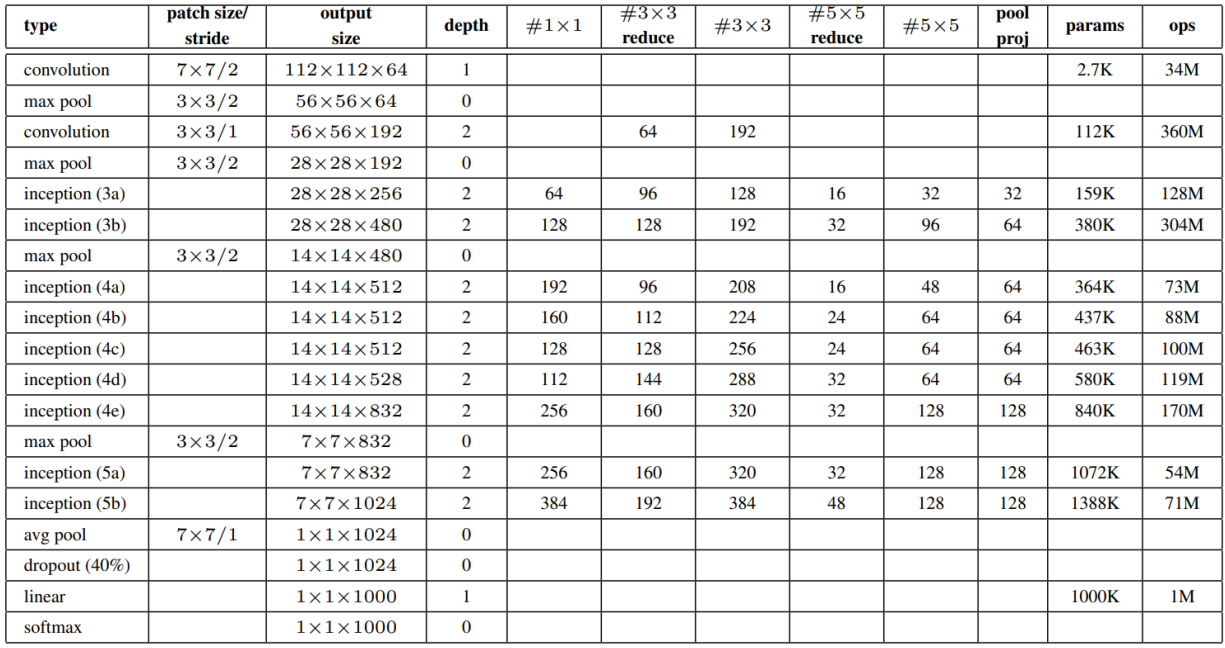
- 上图中Inception模块图与表的对应理解。上表中每行代表一层信息,带#列的每个数字代表卷积核的个数即Inception模块的参数信息,如上图中Inception模块层结构为:输入28 * 28 * 192的图片,首选,经过64个大小为1 * 1的卷积核的卷积层;其次,先经过96个大小为3 * 3的卷积核的卷积层降维,再经过128个大小为3 * 3的卷积核的卷积层;然后,先经过16个大小为 5 * 5的卷积核的卷积层降维,再经过32个大小为5 * 5的卷积核的卷积层;最后,先经过192个大小为 3 * 3的最大池化层,再经过32个大小为1 * 1的卷积核的卷积层;然后再将上面四个部分进行拼接。
- 代码小知识:TensorFlow中 padding = ‘same’时,输出图像的长和宽=输入图像 / 步长 (结果向上取整),因此,如果步长为1,卷积、池化操作不改变图像的长宽
- 辅助分类器结构

; 4.3 GoogleNet网络结构
- 网络结构图

- 表格形式的网络结构表示
; 4.4 GoogleNet代码实现
import tensorflow as tffrom tensorflow.keras.preprocessing.image import ImageDataGeneratorimport numpy as npimport pandas as pdimport matplotlib.pyplot as plttrain_dir = 'sat1/train'test_dir = 'sat1/val'batch_size = 32img_size = 224train_gen = ImageDataGenerator(rescale=1 / 255, horizontal_flip=True)test_gen = ImageDataGenerator(rescale=1 / 255)train_images = train_gen.flow_from_directory(directory=train_dir, target_size=(img_size, img_size), batch_size=batch_size, shuffle=True, class_mode='categorical')test_images = train_gen.flow_from_directory(directory=test_dir, target_size=(img_size, img_size), batch_size=batch_size, shuffle=False, class_mode='categorical')classes = train_images.class_indicesprint("===============================类别索引============================")print(classes)def Inception(con1x1, con3x3reduce, con3x3, con5x5reduce, con5x5, pool_proj, input_): inputs = tf.keras.layers.Input(shape=input_.shape[1:]) x1 = tf.keras.layers.Conv2D(filters=con1x1, kernel_size=(1, 1), activation='relu')(inputs) x21 = tf.keras.layers.Conv2D(filters=con3x3reduce, kernel_size=(1, 1), activation='relu')(inputs) x22 = tf.keras.layers.Conv2D(filters=con3x3, kernel_size=(3, 3), padding='same', activation='relu')(x21) x31 = tf.keras.layers.Conv2D(filters=con5x5reduce, kernel_size=1, activation='relu')(inputs) x32 = tf.keras.layers.Conv2D(filters=con5x5, kernel_size=5, padding='same', activation='relu')(x31) x41 = tf.keras.layers.MaxPooling2D(pool_size=(3, 3), padding='same', strides=1)(inputs) x42 = tf.keras.layers.Conv2D(filters=pool_proj, kernel_size=1, activation='relu')(x41) outputs = tf.concat((x1, x22, x32, x42), axis=-1) return tf.keras.Model(inputs=inputs, outputs=outputs)def InceptionAux(num_classes, input_): inputs = tf.keras.layers.Input(shape=input_.shape[1:]) x = tf.keras.layers.AvgPool2D(pool_size=5, strides=3)(inputs) x = tf.keras.layers.Conv2D(128, kernel_size=1, activation="relu")(x) x = tf.keras.layers.Flatten()(x) x = tf.keras.layers.Dropout(rate=0.7)(x) x = tf.keras.layers.Dense(1024, activation="relu")(x) x = tf.keras.layers.Dropout(rate=0.7)(x) x = tf.keras.layers.Dense(num_classes)(x) return tf.keras.Model(inputs=inputs, outputs=x)def GoogleNet(): input_image = tf.keras.layers.Input(shape=(224, 224, 3)) x = tf.keras.layers.Conv2D(filters=64, kernel_size=7, strides=2, padding='same', activation='relu')(input_image) x = tf.keras.layers.MaxPool2D(pool_size=3, strides=2, padding="same")(x) x = tf.keras.layers.Conv2D(64, kernel_size=1, activation="relu")(x) x = tf.keras.layers.Conv2D(192, kernel_size=3, padding="same", activation="relu")(x) x = tf.keras.layers.MaxPool2D(pool_size=3, strides=2, padding="same")(x) x = Inception(64, 96, 128, 16, 32, 32, x)(x) x = Inception(128, 128, 192, 32, 96, 64, x)(x) x = tf.keras.layers.MaxPool2D(pool_size=3, strides=2, padding="same")(x) x = Inception(192, 96, 208, 16, 48, 64, x)(x) aux11 = InceptionAux(5, x)(x) aux1 = tf.keras.layers.Softmax(name="aux_1")(aux11) x = Inception(160, 112, 224, 24, 64, 64, x)(x) x = Inception(128, 128, 256, 24, 64, 64, x)(x) x = Inception(112, 144, 288, 32, 64, 64, x)(x) aux22 = InceptionAux(5, x)(x) aux2 = tf.keras.layers.Softmax(name="aux_2")(aux22) x = Inception(256, 160, 320, 32, 128, 128, x)(x) x = tf.keras.layers.MaxPool2D(pool_size=3, strides=2, padding="same")(x) x = Inception(256, 160, 320, 32, 128, 128, x)(x) x = Inception(384, 192, 384, 48, 128, 128, x)(x) x = tf.keras.layers.AvgPool2D(pool_size=7, strides=1)(x) x = tf.keras.layers.Flatten()(x) x = tf.keras.layers.Dropout(rate=0.4)(x) x = tf.keras.layers.Dense(5)(x) aux3 = tf.keras.layers.Softmax(name="aux_3")(x) model = tf.keras.models.Model(inputs=input_image, outputs=[aux1, aux2, aux3]) return modelmodelNet = GoogleNet()modelNet.compile(optimizer=tf.keras.optimizers.Adam(learning_rate=0.0005), loss='categorical_crossentropy', metrics=['acc'])history = modelNet.fit(train_images, epochs=20, validation_data=test_images)plt.plot(history.epoch, history.history.get('aux_3_acc'))plt.plot(history.epoch, history.history.get('val_aux_3_acc'))modelNet.evaluate(test_images)modelNet.save('sat5.h5')4.5 GoogleNet网络的发展(Inception V2 V3 V4)

; 5. ResNet实现遥感图像分类
5.1 数据集介绍
与AlexNet网络中使用的数据集一样
5.2 ResNet网络创新
第一. 该网络发现了通过残差结构避免网络退化现象,神经网络的”深度”首次突破了100层。
第二. 采用Batch Normalization 批量归一化,避免梯度消失和爆炸,使得训练更稳定。

- Batch Normalization 批量归一化:每一层输入的时候,先做一个归一化处理,然后再进入网络的下一层。这个输入值的分布强行拉回到均值为0方差为1。避免梯度消失和爆炸,训练更稳定。
- 退化现象:网络层数的增多,训练集loss逐渐下降,然后趋于饱和。当你再增加网络深度的话,训练集loss反而增大。

- 捷径分支:输入层和输出层之和可以避免网络退化(我的理解是,和间接得到整体残差,即去掉输入和输出之间的无用层)
[En]
Shortcut branch: the summation of the input layer and the output layer can avoid network degradation (my understanding is that the sum indirectly gets the overall residual, that is, the useless layer between input and output is removed)*

- 基于捷径分支的思想,ResNet18 和ResNet34的残差模块结构如下

上图中残差结构的具体代码实现[En]
The specific code implementation of the residual structure in the figure above
def BasicBlock(filter_num, strides, _inputs): x = tf.keras.layers.Conv2D(filters=filter_num, kernel_size=3, strides=strides, padding='same')(_inputs) x = tf.keras.layers.BatchNormalization()(x) x = tf.keras.layers.Activation('relu')(x) x = tf.keras.layers.Conv2D(filter_num, kernel_size=3, strides=1, padding='same')(x) x = tf.keras.layers.BatchNormalization()(x) if strides != 1: y = tf.keras.layers.Conv2D(filters=filter_num, kernel_size=1, strides=strides)(_inputs) y = tf.keras.layers.BatchNormalization()(y) else: y = _inputs output = tf.keras.layers.add([x, y]) output = tf.keras.layers.Activation('relu')(output) return output- 基于捷径分支的思想,ResNet50和ResNet101及ResNet152的残差模块结构如下

上图中残差结构的具体代码实现[En]
The specific code implementation of the residual structure in the figure above
def BottleNeck(filter_num, strides, _inputs, down=False): x = tf.keras.layers.Conv2D(filters=filter_num, kernel_size=1, strides=1, padding='same')(_inputs) x = tf.keras.layers.BatchNormalization()(x) x = tf.keras.layers.Activation('relu')(x) x = tf.keras.layers.Conv2D(filters=filter_num, kernel_size=3, strides=strides, padding='same')(x) x = tf.keras.layers.BatchNormalization()(x) x = tf.keras.layers.Activation('relu')(x) x = tf.keras.layers.Conv2D(filters=filter_num * 4, kernel_size=1, strides=1, padding='same')(x) x = tf.keras.layers.BatchNormalization()(x) if strides != 1 or down == True: y = tf.keras.layers.Conv2D(filters=filter_num * 4, kernel_size=1, strides=strides)(_inputs) y = tf.keras.layers.BatchNormalization()(y) else: y = _inputs output = tf.keras.layers.add([x, y]) output = tf.keras.layers.Activation('relu')(output) return output5.3 ResNet网络结构

上表解释:
- 无论是ResNet18(有18层网络),还是其它都先经过一层卷积(卷积核大小为7 * 7,卷积核个数为64个,步长为2);然后再经过一层最大池化层。
- 然后每一个大括号代表一个残差结构(有2个或者3个卷积操作组成),大括号旁边的数字代表该残差结构重复的个数,同时要注意cov3_x,cov4_x,cov5_x中的第一层卷积的步长为2,其余全为1
- 最后再经过一层均值池化和全连接层,完成分类
如ResNet18的网络结构实现代码
    input_image = tf.keras.layers.Input(shape=(224, 224, 3))

    x = tf.keras.layers.Conv2D(64, kernel_size=7, strides=2, padding="same")(input_image)
    x = tf.keras.layers.BatchNormalization()(x)
    x = tf.keras.layers.Activation('relu')(x)

    x = tf.keras.layers.MaxPool2D(pool_size=3, strides=2, padding="same")(x)

    x = BasicBlock(64, strides=1, _inputs=x)
    x = BasicBlock(64, strides=1, _inputs=x)

    x = BasicBlock(128, strides=2, _inputs=x)
    x = BasicBlock(128, strides=1, _inputs=x)

    x = BasicBlock(256, strides=2, _inputs=x)
    x = BasicBlock(256, strides=1, _inputs=x)

    x = BasicBlock(512, strides=2, _inputs=x)
    x = BasicBlock(512, strides=1, _inputs=x)

    x = tf.keras.layers.GlobalAveragePooling2D()(x)

    x = tf.keras.layers.Dense(5, activation='softmax')(x)

    model = tf.keras.models.Model(inputs=input_image, outputs=x)
    return model
5.4 ResNet代码实现
ResNet-18和ResNet-50代码实现,其它ResNet代码实现类似
import tensorflow as tf
from tensorflow.keras.preprocessing.image import ImageDataGenerator

import matplotlib.pyplot as plt

train_dir = 'sat1/train'
test_dir = 'sat1/val'

im_size = 224
batch_size = 32

train_images = ImageDataGenerator(rescale=1 / 255, horizontal_flip=True)
test_images = ImageDataGenerator(rescale=1 / 255)

train_gen = train_images.flow_from_directory(directory=train_dir,
                                             batch_size=batch_size,
                                             shuffle=True,
                                             target_size=(im_size, im_size),
                                             class_mode='categorical')

val_gen = test_images.flow_from_directory(directory=test_dir,
                                          batch_size=batch_size,
                                          shuffle=False,
                                          target_size=(im_size, im_size),
                                          class_mode='categorical')

def BasicBlock(filter_num, strides, _inputs):
    x = tf.keras.layers.Conv2D(filters=filter_num, kernel_size=3, strides=strides, padding='same')(_inputs)
    x = tf.keras.layers.BatchNormalization()(x)
    x = tf.keras.layers.Activation('relu')(x)
    x = tf.keras.layers.Conv2D(filter_num, kernel_size=3, strides=1, padding='same')(x)
    x = tf.keras.layers.BatchNormalization()(x)

    if strides != 1:
        y = tf.keras.layers.Conv2D(filters=filter_num, kernel_size=1, strides=strides)(_inputs)
        y = tf.keras.layers.BatchNormalization()(y)
    else:
        y = _inputs

    output = tf.keras.layers.add([x, y])
    output = tf.keras.layers.Activation('relu')(output)

    return output

def ResNet18():
    input_image = tf.keras.layers.Input(shape=(224, 224, 3))
    x = tf.keras.layers.Conv2D(64, kernel_size=7, strides=2, padding="same")(input_image)
    x = tf.keras.layers.BatchNormalization()(x)
    x = tf.keras.layers.Activation('relu')(x)
    x = tf.keras.layers.MaxPool2D(pool_size=3, strides=2, padding="same")(x)

    x = BasicBlock(64, strides=1, _inputs=x)
    x = BasicBlock(64, strides=1, _inputs=x)

    x = BasicBlock(128, strides=2, _inputs=x)
    x = BasicBlock(128, strides=1, _inputs=x)

    x = BasicBlock(256, strides=2, _inputs=x)
    x = BasicBlock(256, strides=1, _inputs=x)

    x = BasicBlock(512, strides=2, _inputs=x)
    x = BasicBlock(512, strides=1, _inputs=x)

    x = tf.keras.layers.GlobalAveragePooling2D()(x)

    x = tf.keras.layers.Dense(5, activation='softmax')(x)

    model = tf.keras.models.Model(inputs=input_image, outputs=x)
    return model

def BottleNeck(filter_num, strides, _inputs, down=False):
    x = tf.keras.layers.Conv2D(filters=filter_num, kernel_size=1, strides=1, padding='same')(_inputs)
    x = tf.keras.layers.BatchNormalization()(x)
    x = tf.keras.layers.Activation('relu')(x)
    x = tf.keras.layers.Conv2D(filters=filter_num, kernel_size=3, strides=strides, padding='same')(x)
    x = tf.keras.layers.BatchNormalization()(x)
    x = tf.keras.layers.Activation('relu')(x)
    x = tf.keras.layers.Conv2D(filters=filter_num * 4, kernel_size=1, strides=1, padding='same')(x)
    x = tf.keras.layers.BatchNormalization()(x)

    if strides != 1 or down == True:
        y = tf.keras.layers.Conv2D(filters=filter_num * 4, kernel_size=1, strides=strides)(_inputs)
        y = tf.keras.layers.BatchNormalization()(y)
    else:
        y = _inputs

    output = tf.keras.layers.add([x, y])
    output = tf.keras.layers.Activation('relu')(output)

    return output

def ResNet50():
    input_image = tf.keras.layers.Input(shape=(224, 224, 3))
    x = tf.keras.layers.Conv2D(64, kernel_size=7, strides=2, padding="same")(input_image)
    x = tf.keras.layers.BatchNormalization()(x)
    x = tf.keras.layers.MaxPool2D(pool_size=3, strides=2, padding="same")(x)

    x = BottleNeck(filter_num=64, strides=1, _inputs=x, down=True)
    x = BottleNeck(filter_num=64, strides=1, _inputs=x)
    x = BottleNeck(filter_num=64, strides=1, _inputs=x)

    x = BottleNeck(filter_num=128, strides=2, _inputs=x)
    x = BottleNeck(filter_num=128, strides=1, _inputs=x)
    x = BottleNeck(filter_num=128, strides=1, _inputs=x)
    x = BottleNeck(filter_num=128, strides=1, _inputs=x)

    x = BottleNeck(filter_num=256, strides=2, _inputs=x)
    x = BottleNeck(filter_num=256, strides=1, _inputs=x)
    x = BottleNeck(filter_num=256, strides=1, _inputs=x)
    x = BottleNeck(filter_num=256, strides=1, _inputs=x)
    x = BottleNeck(filter_num=256, strides=1, _inputs=x)
    x = BottleNeck(filter_num=256, strides=1, _inputs=x)

    x = BottleNeck(filter_num=512, strides=2, _inputs=x)
    x = BottleNeck(filter_num=512, strides=1, _inputs=x)
    x = BottleNeck(filter_num=512, strides=1, _inputs=x)

    x = tf.keras.layers.GlobalAveragePooling2D()(x)
    x = tf.keras.layers.Dense(5, activation='softmax')(x)

    model = tf.keras.models.Model(inputs=input_image, outputs=x)
    return model

model = ResNet18()
model.summary()

model.compile(optimizer=tf.keras.optimizers.Adam(learning_rate=0.0005),
              loss='categorical_crossentropy',
              metrics=['acc'])

history = model.fit(train_gen, epochs=10, validation_data=val_gen)

plt.plot(history.epoch, history.history.get('acc'))
plt.plot(history.epoch, history.history.get('val_acc'))

model.evaluate(val_gen)
Original: https://blog.csdn.net/qq_34720818/article/details/121169682
Author: Mekeater
Title: 基于卷积神经网络的图像识别技术从入门到深爱(理论思想与代码实践齐飞)
原创文章受到原创版权保护。转载请注明出处:https://www.johngo689.com/514128/
转载文章受原作者版权保护。转载请注明原作者出处!