《Deep Learning With Python second edition》英文版读书笔记：第十一章DL for text: NLP、Transformer、Seq2Seq

文章目录

*
– 第十一章：Deep learning for text
–
+ 11.1 Natural language processing: The bird’s eye view
+ 11.2 Preparing text data
+ 11.3 Two approaches for representing groups of words:Sets and sequences
+ 11.4 The Transformer architecture
+
* 11.4.3 The Transformer encoder
+ 11.5 Beyond text classification: Sequence-to-sequence learning
+
* 11.5.1 A machine translation example
* 11.5.2 Sequence-to-sequence learning with RNNs
* 11.5.3 Sequence-to-sequence learning with Transformer
+ Summary
– 后记

写在前面，本文是阅读python深度学习第二版的读书笔记，仅用于个人学习使用。另外，截至2022年3月18日，距离该版的英文版发布已经将近5个月，国内还未翻译过来。这里的启发是什么呢？学好英文，接触一手的资料！

; 第十一章：Deep learning for text

本章的主要内容

This chapter covers
 Preprocessing text data for machine learning
applications
 Bag-of-words approaches and sequence-modeling
approaches for text processing
 The Transformer architecture
 Sequence-to-sequence learning

11.1 Natural language processing: The bird’s eye view

编程语言和自然语言不同

In computer science, we refer to human languages, like English or Mandarin, as
“natural” languages, to distinguish them from languages that were designed for
machines, like Assembly, LISP, or XML. Every machine language was designed: its
starting point was a human engineer writing down a set of formal rules to describe
what statements you could make in that language and what they meant. Rules came
first, and people only started using the language once the rule set was complete.

With human language, it’s the reverse: usage comes first, rules arise later. Natural
language was shaped by an evolution process, much like biological organisms—
that’s what makes it “natural.” Its “rules,” like the grammar of English, were formalized
after the fact and are often ignored or broken by its users. As a result, while machine-readable language is highly structured and rigorous, using precise syntactic
rules to weave together exactly defined concepts from a fixed vocabulary, natural language
is messy—ambiguous, chaotic, sprawling, and constantly in flux.

handcraft complex sets of rules to perform machine translation 行不通

Creating algorithms that can make sense of natural language is a big deal: language,
and in particular text, underpins most of our communications and our cultural
production. The internet is mostly text. Language is how we store almost all of
our knowledge. Our very thoughts are largely built upon language. However, the ability
to understand natural language has long eluded machines. Some people once
naively thought that you could simply write down the “rule set of English,” much like
one can write down the rule set of LISP. Early attempts to build natural language processing
(NLP) systems were thus made through the lens of “applied linguistics.” Engineers
and linguists would handcraft complex sets of rules to perform basic machine
translation or create simple chatbots—like the famous ELIZA program from the
1960s, which used pattern matching to sustain very basic conversation. But language is
a rebellious thing: it’s not easily pliable to formalization. After several decades of
effort, the capabilities of these systems remained disappointing.

统计NLP方法

Handcrafted rules held out as the dominant approach well into the 1990s. But
starting in the late 1980s, faster computers and greater data availability started making
a better alternative viable. When you find yourself building systems that are big piles
of ad hoc rules, as a clever engineer, you’re likely to start asking: “Could I use a corpus
of data to automate the process of finding these rules? Could I search for the rules
within some kind of rule space, instead of having to come up with them myself?” And
just like that, you’ve graduated to doing machine learning. And so, in the late 1980s,
we started seeing machine learning approaches to natural language processing. The
earliest ones were based on decision trees—the intent was literally to automate the
development of the kind of if/then/else rules of previous systems. Then statistical
approaches started gaining speed, starting with logistic regression. Over time, learned
parametric models fully took over, and linguistics came to be seen as more of a hindrance
than a useful tool. Frederick Jelinek, an early speech recognition researcher,
joked in the 1990s: “Every time I fire a linguist, the performance of the speech recognizer
goes up.”

下面是modern NLP的一些任务：

That’s what modern NLP is about: using machine learning and large datasets to
give computers the ability not to understand language, which is a more lofty goal, but
to ingest a piece of language as input and return something useful, like predicting the
following:
 “What’s the topic of this text?” (text classification)
 “Does this text contain abuse?” (content filtering)
 “Does this text sound positive or negative?” (sentiment analysis)
 “What should be the next word in this incomplete sentence?” (language modeling)
 “How would you say this in German?” (translation)
 “How would you summarize this article in one paragraph?” (summarization)
 etc.

对NLP的简单介绍: 就是模式识别在texts中的应用

Of course, keep in mind throughout this chapter that the text-processing models you
will train won’t possess a human-like understanding of language; rather, they simply
look for statistical regularities in their input data, which turns out to be sufficient to
perform well on many simple tasks. In much the same way that computer vision is pattern
recognition applied to pixels, NLP is pattern recognition applied to words, sentences,
and paragraphs.

recurrent neural networks：递归神经网路

介绍一下近些年NLP模型的发展,现在用的多的是transformer

The toolset of NLP—decision trees, logistic regression—only saw slow evolution
from the 1990s to the early 2010s. Most of the research focus was on feature engineering.

When I won my first NLP competition on Kaggle in 2013, my model was, you
guessed it, based on decision trees and logistic regression. However, around 2014–
2015, things started changing at last. Multiple researchers began to investigate the
language-understanding capabilities of recurrent neural networks, in particular LSTM—
a sequence-processing algorithm from the late 1990s that had stayed under the radar
until then.

In early 2015, Keras made available the first open source, easy-to-use implementation
of LSTM, just at the start of a massive wave of renewed interest in recurrent neural
networks—until then, there had only been “research code” that couldn’t be readily
reused. Then from 2015 to 2017, recurrent neural networks dominated the booming
NLP scene. Bidirectional LSTM models, in particular, set the state of the art on many important tasks, from summarization to question-answering to machine translation.

Finally, around 2017–2018, a new architecture rose to replace RNNs: the Transformer,
which you will learn about in the second half of this chapter. Transformers
unlocked considerable progress across the field in a short period of time, and today
most NLP systems are based on them.

Let’s dive into the details. This chapter will take you from the very basics to doing
machine translation with a Transformer.

11.2 Preparing text data

下面是一些重要的概念：tokens，indexing all tokens

Deep learning models, being differentiable functions, can only process numeric tensors:
they can’t take raw text as input. Vectorizing text is the process of transforming
text into numeric tensors. Text vectorization processes come in many shapes and
forms, but they all follow the same template (see figure 11.1):
 First, you standardize the text to make it easier to process, such as by converting
it to lowercase or removing punctuation.

 You split the text into units (called tokens), such as characters, words, or groups
of words. This is called tokenization.

 You convert each such token into a numerical vector. This will usually involve
first indexing all tokens present in the data.

Let’s review each of these steps.

下图就是整个初始化text的过程

11.2.1 Text standardization

Consider these two sentences:
 “sunset came. i was staring at the Mexico sky. Isnt nature splendid??”
 “Sunset came; I stared at the México sky. Isn’t nature splendid?”
They’re very similar—in fact, they’re almost identical. Yet, if you were to convert them
to byte strings, they would end up with very different representations, because “i” and
“I” are two different characters, “Mexico” and “México” are two different words, “isnt”
isn’t “isn’t,” and so on. A machine learning model doesn’t know a priori that “i” and
“I” are the same letter, that “é” is an “e” with an accent, or that “staring” and “stared”
are two forms of the same verb.

Text standardization is a basic form of feature engineering that aims to erase
encoding differences that you don’t want your model to have to deal with. It’s not
exclusive to machine learning, either—you’d have to do the same thing if you were
building a search engine.

简单处理

One of the simplest and most widespread standardization schemes is “convert to
lowercase and remove punctuation characters.” Our two sentences would become
 “sunset came i was staring at the mexico sky isnt nature splendid”
 “sunset came i stared at the méxico sky isnt nature splendid”

还有：stemming这个技巧，把一个单词的不同形式编码为a single shared representation

Much closer already. Another common transformation is to convert special characters
to a standard form, such as replacing “é” with “e,” “æ” with “ae,” and so on. Our token
“méxico” would then become “mexico”.

Lastly, a much more advanced standardization pattern that is more rarely used in a
machine learning context is stemming: converting variations of a term (such as different
conjugated forms of a verb) into a single shared representation, like turning
“caught” and “been catching” into “[catch]” or “cats” into “[cat]”. With stemming,
“was staring” and “stared” would become something like “[stare]”, and our two similar
sentences would finally end up with an identical encoding:
 “sunset came i [stare] at the mexico sky isnt nature splendid”

标准化的好处

With these standardization techniques, your model will require less training data and
will generalize better—it won’t need abundant examples of both “Sunset” and “sunset”
to learn that they mean the same thing, and it will be able to make sense of “México”
even if it has only seen “mexico” in its training set. Of course, standardization may
also erase some amount of information, so always keep the context in mind: for
instance, if you’re writing a model that extracts questions from interview articles, it
should definitely treat “?” as a separate token instead of dropping it, because it’s a useful
signal for this specific task.

11.2.2 Text splitting (tokenization)

Once your text is standardized, you need to break it up into units to be vectorized
(tokens), a step called tokenization. You could do this in three different ways:
 Word-level tokenization—Where tokens are space-separated (or punctuationseparated)
substrings. A variant of this is to further split words into subwords
when applicable—for instance, treating “staring” as “star+ing” or “called” as
“call+ed.”
 N-gram tokenization—Where tokens are groups of N consecutive words. For
instance, “the cat” or “he was” would be 2-gram tokens (also called bigrams).

 Character-level tokenization—Where each character is its own token. In practice,
this scheme is rarely used, and you only really see it in specialized contexts, like
text generation or speech recognition.

两类模型：

• sequence models: care about words order, using word-level tokenization
• bag-of-words models: discard order of words, such as N-grams models

In general, you’ll always use either word-level or N-gram tokenization. There are two
kinds of text-processing models: those that care about word order, called sequence models,
and those that treat input words as a set, discarding their original order, called
bag-of-words models. If you’re building a sequence model, you’ll use word-level tokenization,
and if you’re building a bag-of-words model, you’ll use N-gram tokenization.

N-grams are a way to artificially inject a small amount of local word order information
into the model. Throughout this chapter, you’ll learn more about each type of model
and when to use them.

下面是对N-grams和bag-of-words的解释

Understanding N-grams and bag-of-words
Word N-grams are groups of N (or fewer) consecutive words that you can extract from
a sentence. The same concept may also be applied to characters instead of words.

Here’s a simple example. Consider the sentence “the cat sat on the mat.” It may be
decomposed into the following set of 2-grams:
{“the”, “the cat”, “cat”, “cat sat”, “sat”,
“sat on”, “on”, “on the”, “the mat”, “mat”}
It may also be decomposed into the following set of 3-grams:
{“the”, “the cat”, “cat”, “cat sat”, “the cat sat”,
“sat”, “sat on”, “on”, “cat sat on”, “on the”,
“sat on the”, “the mat”, “mat”, “on the mat”}
Such a set is called a bag-of-2-grams or bag-of-3-grams, respectively. The term “bag”
here refers to the fact that you’re dealing with a set of tokens rather than a list or
sequence: the tokens have no specific order. This family of tokenization methods is
called bag-of-words (or bag-of-N-grams).

Because bag-of-words isn’t an order-preserving tokenization method (the tokens generated
are understood as a set, not a sequence, and the general structure of the sentences
is lost), it tends to be used in shallow language-processing models rather than
in deep learning models. Extracting N-grams is a form of feature engineering, and
deep learning sequence models do away with this manual approach, replacing it with
hierarchical feature learning. One-dimensional convnets, recurrent neural networks,
and Transformers are capable of learning representations for groups of words and
characters without being explicitly told about the existence of such groups, by looking
at continuous word or character sequences.

11.2.3 Vocabulary indexing

Once your text is split into tokens, you need to encode each token into a numerical
representation. You could potentially do this in a stateless way, such as by hashing each
token into a fixed binary vector, but in practice, the way you’d go about it is to build
an index of all terms found in the training data (the “vocabulary”), and assign a
unique integer to each entry in the vocabulary.

不用管用的少的words

Note that at this step it’s common to restrict the vocabulary to only the top 20,000 or
30,000 most common words found in the training data. Any text dataset tends to feature
an extremely large number of unique terms, most of which only show up once or
twice—indexing those rare terms would result in an excessively large feature space,
where most features would have almost no information content.

记得使用OOV index来记录上述的越界单词（很少用的单词）

Remember when you were training your first deep learning models on the IMDB
dataset in chapters 4 and 5? The data you were using from keras.datasets.imdb was
already preprocessed into sequences of integers, where each integer stood for a given
word. Back then, we used the setting num_words=10000, in order to restrict our vocabulary
to the top 10,000 most common words found in the training data.

Now, there’s an important detail here that we shouldn’t overlook: when we look
up a new token in our vocabulary index, it may not necessarily exist. Your training
data may not have contained any instance of the word “cherimoya” (or maybe you
excluded it from your index because it was too rare), so doing token_index =
vocabulary[“cherimoya”] may result in a KeyError. To handle this, you should use
an “out of vocabulary” index (abbreviated as OOV index)—a catch-all for any token
that wasn’t in the index. It’s usually index 1: you’re actually doing token_index =
vocabulary.get(token, 1). When decoding a sequence of integers back into words,
you’ll replace 1 with something like “[UNK]” (which you’d call an “OOV token”).

索引1表示OOV

索引0表示not a word

短的序列需要padded to 最长序列的长度

“Why use 1 and not 0?” you may ask. That’s because 0 is already taken. There are
two special tokens that you will commonly use: the OOV token (index 1), and the
mask token (index 0). While the OOV token means “here was a word we did not recognize,”
the mask token tells us “ignore me, I’m not a word.” You’d use it in particular to
pad sequence data: because data batches need to be contiguous, all sequences in a
batch of sequence data must have the same length, so shorter sequences should be
padded to the length of the longest sequence. If you want to make a batch of data with
the sequences [5, 7, 124, 4, 89] and [8, 34, 21], it would have to look like this:

[[5, 7, 124, 4, 89]
[8, 34, 21, 0, 0]]

The batches of integer sequences for the IMDB dataset that you worked with in chapters
4 and 5 were padded with zeros in this way.

11.2.4 Using the TextVectorization layer

Every step I’ve introduced so far would be very easy to implement in pure Python.

Maybe you could write something like this:

python中self相当于java中的this，表示当前类的对象，可以调用当前类中的方法和属性。

import string

class Vectorizer:

    def standardize(self, text):
        text = text.lower()
        return "".join(char for char in text if char not in string.punctuation)

    def tokenize(self, text):
        text = self.standardize(text)
        return text.split()

    def make_vocabulary(self, dataset):
        self.vocabulary = {"": 0, "[UNK]": 1}
        for text in dataset:
            text = self.standardize(text)
            tokens = self.tokenize(text)
            for token in tokens:
                if token not in self.vocabulary:
                    self.vocabulary[token] = len(self.vocabulary)

        self.inverse_vocabulary = dict(
            (v, k) for k, v in self.vocabulary.items())

    def encode(self, text):
        text = self.standardize(text)
        tokens = self.tokenize(text)
        return [self.vocabulary.get(token, 1) for token in tokens]

    def decode(self, int_sequence):
        return " ".join(
            self.inverse_vocabulary.get(i, "[UNK]") for i in int_sequence)

vectorizer = Vectorizer()
dataset = [
    "I write, erase, rewrite",
    "Erase again, and then",
    "A poppy blooms.",
]
vectorizer.make_vocabulary(dataset)

test_sentence = "I write, rewrite, and still rewrite again"
encoded_sentence = vectorizer.encode(test_sentence)
print(encoded_sentence)

decoded_sentence = vectorizer.decode(encoded_sentence)
print(decoded_sentence)

https://www.runoob.com/python/att-dictionary-get.html ： python dict.get() 方法的解释

get(token, 1)的意思是如果没有查找到，返回设置的1；如果是get(token)，在哈希表中如果没有查找到的话，返回默认的None。

以上是自己处理的过程，下面使用Keras TextVectorization

However, using something like this wouldn’t be very performant. In practice, you’ll
work with the Keras TextVectorization layer, which is fast and efficient and can be
dropped directly into a tf.data pipeline or a Keras model.

This is what the TextVectorization layer looks like:

from tensorflow.keras.layers import TextVectorization
text_vectorization = TextVectorization(
    output_mode="int",
)

默认的，TextVectorization layer自动standardize and tokenize

By default, the TextVectorization layer will use the setting “convert to lowercase and
remove punctuation” for text standardization, and “split on whitespace” for tokenization.

But importantly, you can provide custom functions for standardization and tokenization,
which means the layer is flexible enough to handle any use case.

Note that such custom functions should operate on tf.string tensors, not regular Python
strings! For instance, the default layer behavior is equivalent to the following:

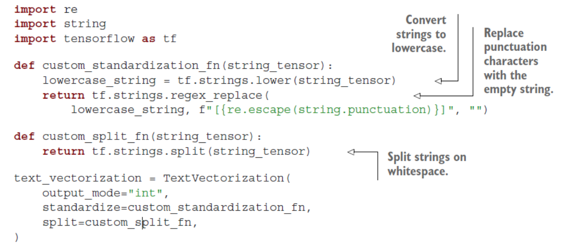
标准化

import re
import string
import tensorflow as tf

def custom_standardization_fn(string_tensor):
    lowercase_string = tf.strings.lower(string_tensor)
    return tf.strings.regex_replace(
        lowercase_string, f"[{re.escape(string.punctuation)}]", "")

def custom_split_fn(string_tensor):
    return tf.strings.split(string_tensor)

text_vectorization = TextVectorization(
    output_mode="int",
    standardize=custom_standardization_fn,
    split=custom_split_fn,
)

添加index使用adapt方法

To index the vocabulary of a text corpus, just call the adapt() method of the layer
with a Dataset object that yields strings, or just with a list of Python strings:

dataset = [
    "I write, erase, rewrite",
    "Erase again, and then",
    "A poppy blooms.",
]
text_vectorization.adapt(dataset)

对adapt的解释

During adapt(), the layer will build a vocabulary of all string tokens seen in the dataset, sorted by occurance count, with ties broken by sort order of the tokens (high to low).

可以使用get_vocabulary()方法检索词汇

Note that you can retrieve the computed vocabulary via get_vocabulary()—this can
be useful if you need to convert text encoded as integer sequences back into words.

The first two entries in the vocabulary are the mask token (index 0) and the OOV
token (index 1). Entries in the vocabulary list are sorted by frequency, so with a realworld
dataset, very common words like “the” or “a” would come first.

展示词汇

text_vectorization.get_vocabulary()

output

['',
 '[UNK]',
 'erase',
 'write',
 'then',
 'rewrite',
 'poppy',
 'i',
 'blooms',
 'and',
 'again',
 'a']

测试一下

vocabulary = text_vectorization.get_vocabulary()
test_sentence = "I write, rewrite, and still rewrite again hello a an great"
encoded_sentence = text_vectorization(test_sentence)
print(encoded_sentence)

output

tf.Tensor([ 7  3  5  9  1  5 10  1 11  1  1], shape=(11,), dtype=int64)

inverse_vocab = dict(enumerate(vocabulary))
decoded_sentence = " ".join(inverse_vocab[int(i)] for i in encoded_sentence)
print(decoded_sentence)

output

i write rewrite and [UNK] rewrite again [UNK] a [UNK] [UNK]

TextVectorization是在CPU上跑的

Using the TextVectorization layer in a tf.data pipeline or as part of a model
Importantly, because TextVectorization is mostly a dictionary lookup operation, it
can’t be executed on a GPU (or TPU)—only on a CPU. So if you’re training your model
on a GPU, your TextVectorization layer will run on the CPU before sending its output
to the GPU. This has important performance implications.

有两种方式使用TextVectorization layer

两种方式有很大的区别

There’s an important difference between the two: if the vectorization step is part of
the model, it will happen synchronously with the rest of the model. This means that
at each training step, the rest of the model (placed on the GPU) will have to wait for
the output of the TextVectorization layer (placed on the CPU) to be ready in order
to get to work. Meanwhile, putting the layer in the tf.data pipeline enables you to do asynchronous preprocessing of your data on CPU: while the GPU runs the model
on one batch of vectorized data, the CPU stays busy by vectorizing the next batch of
raw strings.

如果使用GPU训练的话，倾向于使用第一种：tf.data pipeline

So if you’re training the model on GPU or TPU, you’ll probably want to go with the first
option to get the best performance. This is what we will do in all practical examples
throughout this chapter. When training on a CPU, though, synchronous processing is
fine: you will get 100% utilization of your cores regardless of which option you go with.

export to a production environment

Now, if you were to export our model to a production environment, you would want to
ship a model that accepts raw strings as input, like in the code snippet for the second
option above—otherwise you would have to reimplement text standardization and
tokenization in your production environment (maybe in JavaScript?), and you would
face the risk of introducing small preprocessing discrepancies that would hurt the
model’s accuracy. Thankfully, the TextVectorization layer enables you to include
text preprocessing right into your model, making it easier to deploy—even if you were
originally using the layer as part of a tf.data pipeline. In the sidebar “Exporting a
model that processes raw strings,” you’ll learn how to export an inference-only
trained model that incorporates text preprocessing.

11.3 Two approaches for representing groups of words:Sets and sequences

word order

How a machine learning model should represent individual words is a relatively uncontroversial
question: they’re categorical features (values from a predefined set), and we
know how to handle those. They should be encoded as dimensions in a feature space,
or as category vectors (word vectors in this case). A much more problematic question,
however, is how to encode the way words are woven into sentences: word order.

语序很重要，但它与整个句子的意思没有那么直接的关系。

[En]

Word order is important, but it is not so directly related to the meaning of the whole sentence.

The problem of order in natural language is an interesting one: unlike the steps of
a timeseries, words in a sentence don’t have a natural, canonical order. Different languages
order similar words in very different ways. For instance, the sentence structure
of English is quite different from that of Japanese. Even within a given language, you
can typically say the same thing in different ways by reshuffling the words a bit. Even
further, if you fully randomize the words in a short sentence, you can still largely figure
out what it was saying—though in many cases significant ambiguity seems to arise.

Order is clearly important, but its relationship to meaning isn’t straightforward.

下面是几个模型

How to represent word order is the pivotal question from which different kinds of
NLP architectures spring. The simplest thing you could do is just discard order and
treat text as an unordered set of words—this gives you bag-of-words models. You could
also decide that words should be processed strictly in the order in which they appear,
one at a time, like steps in a timeseries—you could then leverage the recurrent models
from the last chapter. Finally, a hybrid approach is also possible: the Transformer architecture is technically order-agnostic, yet it injects word-position information into
the representations it processes, which enables it to simultaneously look at different
parts of a sentence (unlike RNNs) while still being order-aware. Because they take into
account word order, both RNNs and Transformers are called sequence models.

之前NLP主要处理的是词袋模型，直到2015年才逐渐关注顺序模型。

Historically, most early applications of machine learning to NLP just involved
bag-of-words models. Interest in sequence models only started rising in 2015, with the
rebirth of recurrent neural networks. Today, both approaches remain relevant. Let’s
see how they work, and when to leverage which.

We’ll demonstrate each approach on a well-known text classification benchmark:
the IMDB movie review sentiment-classification dataset. In chapters 4 and 5, you
worked with a prevectorized version of the IMDB dataset; now, let’s process the raw
IMDB text data, just like you would do when approaching a new text-classification
problem in the real world.

11.3.1 Preparing the IMDB movie reviews data

Let’s start by downloading the dataset from the Stanford page of Andrew Maas and
uncompressing it:

!curl -O https://ai.stanford.edu/~amaas/data/sentiment/aclImdb_v1.tar.gz
!tar -xf aclImdb_v1.tar.gz

output

  % Total    % Received % Xferd  Average Speed   Time    Time     Time  Current
                                 Dload  Upload   Total   Spent    Left  Speed
100 80.2M  100 80.2M    0     0  48.6M      0  0:00:01  0:00:01 --:--:-- 48.6M

There’s also a train/unsup subdirectory in there, which we don’t need. Let’s
delete it:

!rm -r aclImdb/train/unsup

这是文件结构

aclImdb/
...train/
......pos/
......neg/
...test/
......pos/
......neg/

For instance, the train/pos/ directory contains a set of 12,500 text files, each of which
contains the text body of a positive-sentiment movie review to be used as training data.

The negative-sentiment reviews live in the “neg” directories. In total, there are 25,000
text files for training and another 25,000 for testing.

Take a look at the content of a few of these text files. Whether you’re working with
text data or image data, remember to always inspect what your data looks like before
you dive into modeling it. It will ground your intuition about what your model is actually
doing:

!cat aclImdb/train/pos/4077_10.txt

output

I first saw this back in the early 90s on UK TV, i did like it then but i missed the chance to tape it, many years passed but the film always stuck with me and i lost hope of seeing it TV again, the main thing that stuck with me was the end, the hole castle part really touched me, its easy to watch, has a great story, great music, the list goes on and on, its OK me saying how good it is but everyone will take there own best bits away with them once they have seen it, yes the animation is top notch and beautiful to watch, it does show its age in a very few parts but that has now become part of it beauty, i am so glad it has came out on DVD as it is one of my top 10 films of all time. Buy it or rent it just see it, best viewing is at night alone with drink and food in reach so you don't have to stop the film.<br><br>Enjoy

prepare a validation set

Next, let’s prepare a validation set by setting apart 20% of the training text files in a
new directory, aclImdb/val:

下面的代码可以学习如何从数据集中提取20%作为验证集

[En]

The following code can learn how to take 20% from the dataset as the validation set

import os, pathlib, shutil, random

base_dir = pathlib.Path("aclImdb")
val_dir = base_dir / "val"
train_dir = base_dir / "train"
for category in ("neg", "pos"):
    os.makedirs(val_dir / category)
    files = os.listdir(train_dir / category)
    random.Random(1337).shuffle(files)
    num_val_samples = int(0.2 * len(files))
    val_files = files[-num_val_samples:]
    for fname in val_files:
        shutil.move(train_dir / category / fname,
                    val_dir / category / fname)

如果运行原始书籍附带的代码，则只能运行一次，第二次运行时会出现错误。

[En]

If you run the code that comes with the original book, you can only run it once, and you will get an error when you run it the second time.

      8     files = os.listdir(train_dir / category)
      9     random.Random(1337).shuffle(files)

/usr/lib/python3.7/os.py in makedirs(name, mode, exist_ok)
    221             return
    222     try:
--> 223         mkdir(name, mode)
    224     except OSError:
    225         # Cannot rely on checking for EEXIST, since the operating system

FileExistsError: [Errno 17] File exists: 'aclImdb/val/neg'
</module></ipython-input-32-c888da3ad7e7>

下面是对代码的解释

Remember how, in chapter 8, we used the image_dataset_from_directory utility to
create a batched Dataset of images and their labels for a directory structure? You can
do the exact same thing for text files using the text_dataset_from_directory utility.

Let’s create three Dataset objects for training, validation, and testing:

from tensorflow import keras
batch_size = 32

train_ds = keras.utils.text_dataset_from_directory(
    "aclImdb/train", batch_size=batch_size
)
val_ds = keras.utils.text_dataset_from_directory(
    "aclImdb/val", batch_size=batch_size
)
test_ds = keras.utils.text_dataset_from_directory(
    "aclImdb/test", batch_size=batch_size
)

output

Found 20000 files belonging to 2 classes.

Found 5000 files belonging to 2 classes.

Found 25000 files belonging to 2 classes.

These datasets yield inputs that are TensorFlow tf.string tensors and targets that are
int32 tensors encoding the value “0” or “1.”

Listing 11.2 Displaying the shapes and dtypes of the first batch

for inputs, targets in train_ds:
    print("inputs.shape:", inputs.shape)
    print("inputs.dtype:", inputs.dtype)
    print("targets.shape:", targets.shape)
    print("targets.dtype:", targets.dtype)
    print("inputs[0]:", inputs[0])
    print("targets[0]:", targets[0])
    break

输出结果

inputs.shape: (32,)
inputs.dtype: <dtype: 'string'>
targets.shape: (32,)
targets.dtype: <dtype: 'int32'>
inputs[0]: tf.Tensor(b'Despite being quite far removed from my expectations, I was thoroughly impressed by Dog Bite Dog. I rented it not knowing much about it, but I essentially expected it to be a martial arts/action film in the standard Hong Kong action tradition, of which I am a devoted fan. I ended up getting something entirely different, which is not at all a bad thing. While the film could be classified as such, and there is definitely some good action and hand to hand combat scenes in the film, it is definitely not the primary focus. Its characters are infinitely more important to the film than its fights, a rather uncommon thing in many Hong Kong action movies.<br><br>I was really quite surprised by the intricacy of the characters and character relationships in the film. The lead character, played by Edison Chen (who is really very good), becomes infinitely more complex by the end of the film than I ever thought he would be after watching the first thirty minutes. The police characters also defied my expectations thoroughly. In fact, the stark and honest portrayal of the seldom seen dark side of the police force was quite possible my favorite aspect of the film. I don\'t know that I would say Dog Bite Dog entirely subverts typical notions of bad criminal, good cop, but it certainly distorts them in ways not often seen in film (unfortunately). So many films, especially Hong Kong action films I find, portray police in what is frankly a VERY ignorantly idealized light. This is one of my least favorite things about the genre. I was pleasantly surprised to see that Dog Bite Dog actually had some very unique, and really quite courageous, ideas to present about the police force. There are negotiation scenes in this film that I have never seen the likes of before, and doubt I will ever see again, and am sure I will remember for quite a while. Also, the criminal characters are shown from an interesting perspective as well, there is some documentary footage in the film of Cambodian boys no older than ten being made to fight each other to the death with their bare hands, which I thought was one of the film\'s most powerful and moving moments. It says a lot about the reason these guys are the way they are, rather than simply condemning them. Also, the relationship between Chen\'s character and the girl he meets in the junk yard reveals a lot about his character. It wasn\'t until this element entered the film that I really started to see the film as an emotional experience rather than only a visceral one. There is something about most on screen relationships that doesn\'t quite get through to me, but for some reason this one really did. The actress does an incredible job with this role which I imagine was not easy to play.<br><br>Dog Bite Dog also features some really breathtaking cinematography, all though it is unfortunately rather uneven. There were some moments that I found really striking, particularly in the last segment of the film, but there was also a good deal of camera work that was just OK. Another slight problem I had was with the pacing, which I also felt was uneven. I found a lot of the "looking for a boat" scenes to be a little alienating, all though it quickly picks up after that. The action scenes are short and not too plentiful, but are truly powerful and effecting, particularly towards the end. The fight choreography is honestly not all that impressive for the most part, all though to its credit it is solid and fairly realistic, but the true strength is the emotional content behind the fights. The final scene, while not a marvel of martial artistry or fight choreography, is one of the most powerful final fights I have ever seen, and I\'ve seen quite a few martial arts films.<br><br>I suppose the biggest determining factor of whether or not one will get much out of Dog Bite Dog is whether or not you can connect with the characters. All of them are certainly some of the more flawed characters one is likely to see in a film of any kind, but there was something very human about all of them that I couldn\'t help but be drawn to and really feel for them, particularly Chen\'s girlfriend. I should say that I doubt most people will like the film as much as I did simply because I imagine that most people will not like or care about the characters in the same way, but I still recommend it highly all the same. It is truly a deeply moving and effecting film if you give it a chance.', shape=(), dtype=string)
targets[0]: tf.Tensor(1, shape=(), dtype=int32)
</dtype:></dtype:>

下面是输出第32个batch

for inputs, targets in train_ds:
    print("inputs.shape:", inputs.shape)
    print("inputs.dtype:", inputs.dtype)
    print("targets.shape:", targets.shape)
    print("targets.dtype:", targets.dtype)
    print("inputs[31]:", inputs[31])
    print("targets[31]:", targets[31])
    break

output

inputs.shape: (32,)
inputs.dtype: <dtype: 'string'>
targets.shape: (32,)
targets.dtype: <dtype: 'int32'>
inputs[31]: tf.Tensor(b'"The Brain Machine" will at least put your own brain into overdrive trying to figure out what it\'s all about. Four subjects of varying backgrounds and intelligence level have been selected for an experiment described by one of the researchers as a scientific study of man and environment. Since the only common denominator among them is the fact that they each have no known family should have been a tip off - none of them will be missed.<br><br>The whole affair is supervised by a mysterious creep known only as The General, but it seems he\'s taking his direction from a Senator who wishes to remain anonymous. Good call there on the Senator\'s part. There\'s also a shadowy guard that the camera constantly zooms in on, who later claims he doesn\'t take his direction from the General or \'The Project\'. Too bad he wasn\'t more effective, he was overpowered rather easily before the whole thing went kablooey.<br><br>If nothing else, the film is a veritable treasure trove of 1970\'s technology featuring repeated shots of dial phones, room size computers and a teletype machine that won\'t quit. Perhaps that was the basis of the film\'s alternate title - "Time Warp"; nothing else would make any sense. As for myself, I\'d like to consider a title suggested by the murdered Dr. Krisner\'s experiment titled \'Group Stress Project\'. It applies to the film\'s actors and viewers alike.<br><br>Keep an eye out just above The General\'s head at poolside when he asks an agent for his weapon, a boom mic is visible above his head for a number of seconds.<br><br>You may want to catch this flick if you\'re a die hard Gerald McRaney fan, could he have ever been that young? James Best also appears in a somewhat uncharacteristic role as a cryptic reverend, but don\'t call him Father. For something a little more up his alley, try to get your hands on 1959\'s "The Killer Shrews". That one at least doesn\'t pretend to take itself so seriously.', shape=(), dtype=string)
targets[31]: tf.Tensor(0, shape=(), dtype=int32)
</dtype:></dtype:>

All set. Now let’s try learning something from this data.

11.3.2 Processing words as a set: The bag-of-words approach

不考虑词序

The simplest way to encode a piece of text for processing by a machine learning
model is to discard order and treat it as a set (a “bag”) of tokens. You could either look
at individual words (unigrams), or try to recover some local order information by
looking at groups of consecutive token (N-grams).

SINGLE WORDS (UNIGRAMS) WITH BINARY ENCODING

If you use a bag of single words, the sentence “the cat sat on the mat” becomes
{“cat”, “mat”, “on”, “sat”, “the”}

The main advantage of this encoding is that you can represent an entire text as a single
vector, where each entry is a presence indicator for a given word. For instance,
using binary encoding (multi-hot), you’d encode a text as a vector with as many
dimensions as there are words in your vocabulary—with 0s almost everywhere and
some 1s for dimensions that encode words present in the text. This is what we did
when we worked with text data in chapters 4 and 5. Let’s try this on our task.

具体过程：

First, let’s process our raw text datasets with a TextVectorization layer so that
they yield multi-hot encoded binary word vectors. Our layer will only look at single
words (that is to say, unigrams).

补充multi-hot的知识

Multi-hot encode your lists to turn them into vectors of 0s and 1s. This would
mean, for instance, turning the sequence [8, 5] into a 10,000-dimensional vector
that would be all 0s except for indices 8 and 5, which would be 1s. Then you
could use a Dense layer, capable of handling floating-point vector data, as the
first layer in your model.

补充lambda表达式

lambda [arg1 [, agr2,.....argn]] : expression

可以有很多参数，最后返回的是expression的值

Listing 11.3 Preprocessing our datasets with a TextVectorization layer

text_vectorization = TextVectorization(
    max_tokens=20000,
    output_mode="multi_hot",
)
text_only_train_ds = train_ds.map(lambda x, y: x)
text_vectorization.adapt(text_only_train_ds)

binary_1gram_train_ds = train_ds.map(
    lambda x, y: (text_vectorization(x), y),
    num_parallel_calls=4)
binary_1gram_val_ds = val_ds.map(
    lambda x, y: (text_vectorization(x), y),
    num_parallel_calls=4)
binary_1gram_test_ds = test_ds.map(
    lambda x, y: (text_vectorization(x), y),
    num_parallel_calls=4)

You can try to inspect the output of one of these datasets.

Listing 11.4 Inspecting the output of our binary unigram dataset

for inputs, targets in binary_1gram_train_ds:
    print("inputs.shape:", inputs.shape)
    print("inputs.dtype:", inputs.dtype)
    print("targets.shape:", targets.shape)
    print("targets.dtype:", targets.dtype)
    print("inputs[0]:", inputs[0])
    print("targets[0]:", targets[0])
    break

output

inputs.shape: (32, 20000)
inputs.dtype: <dtype: 'float32'>
targets.shape: (32,)
targets.dtype: <dtype: 'int32'>
inputs[0]: tf.Tensor([1. 1. 1. ... 0. 0. 0.], shape=(20000,), dtype=float32)
targets[0]: tf.Tensor(1, shape=(), dtype=int32)
</dtype:></dtype:>

写可重用的代码

Next, let’s write a reusable model-building function that we’ll use in all of our experiments
in this section.

Listing 11.5 Our model-building utility

from tensorflow import keras
from tensorflow.keras import layers

def get_model(max_tokens=20000, hidden_dim=16):
    inputs = keras.Input(shape=(max_tokens,))
    x = layers.Dense(hidden_dim, activation="relu")(inputs)
    x = layers.Dropout(0.5)(x)
    outputs = layers.Dense(1, activation="sigmoid")(x)
    model = keras.Model(inputs, outputs)
    model.compile(optimizer="rmsprop",
                  loss="binary_crossentropy",
                  metrics=["accuracy"])
    return model

关于keras.Input的理解

tf.keras.Input(
    shape=None, batch_size=None, name=None, dtype=None, sparse=False, tensor=None,
    ragged=False, **kwargs
)

https://devdocs.io/tensorflow~2.4/keras/input

Arguments shape

A shape tuple (integers), not including the batch size. For instance, shape=(32,)

indicates that the expected input will be batches of 32-dimensional vectors. Elements of this tuple can be None; ‘None’ elements represent dimensions where the shape is not known.

为什么有的Keras函数后两个()，能不能从函数的角度解释下? https://blog.csdn.net/ding_programmer/article/details/100178016

Python 函数两括号()() ()(X)的语法含义： https://blog.csdn.net/u013166171/article/details/81292132

关于keras.dropout的理解

https://devdocs.io/tensorflow~2.4/keras/layers/dropout

tf.keras.layers.Dropout(
    rate, noise_shape=None, seed=None, **kwargs
)

解释：为了防止过拟合，dropout根据rate随机置零，其他未置零的数据变成原来的1/(1-rate)倍。

The Dropout layer randomly sets input units to 0 with a frequency of rate at each step during training time, which helps prevent overfitting. Inputs not set to 0 are scaled up by 1/(1 - rate) such that the sum over all inputs is unchanged.

对于keras.layers.dense的理解

https://devdocs.io/tensorflow~2.4/keras/layers/dense

tf.keras.layers.Dense(
    units, activation=None, use_bias=True,
    kernel_initializer='glorot_uniform',
    bias_initializer='zeros', kernel_regularizer=None,
    bias_regularizer=None, activity_regularizer=None, kernel_constraint=None,
    bias_constraint=None, **kwargs
)

含义： Dense implements the operation: output = activation(dot(input, kernel) + bias) where activation is the element-wise activation function passed as the activation argument, kernel is a weights matrix created by the layer, and bias is a bias vector created by the layer (only applicable if use_bias is True).

举例

model = tf.keras.models.Sequential()
model.add(tf.keras.Input(shape=(16,)))
model.add(tf.keras.layers.Dense(32, activation='relu'))

model.add(tf.keras.layers.Dense(32))
model.output_shape
(None, 32)

参数

Arguments units

Positive integer, dimensionality of the output space. activation

Activation function to use. If you don’t specify anything, no activation is applied (ie. “linear” activation: a(x) = x

). use_bias

Boolean, whether the layer uses a bias vector. kernel_initializer

Initializer for the kernel

weights matrix. bias_initializer

Initializer for the bias vector. kernel_regularizer

Regularizer function applied to the kernel

weights matrix. bias_regularizer

Regularizer function applied to the bias vector. activity_regularizer

Regularizer function applied to the output of the layer (its “activation”). kernel_constraint

Constraint function applied to the kernel

weights matrix. bias_constraint

Constraint function applied to the bias vector.

参数和返回值

Input shape:

N-D tensor with shape: (batch_size, ..., input_dim). The most common situation would be a 2D input with shape (batch_size, input_dim).

Output shape:

N-D tensor with shape: (batch_size, ..., units). For instance, for a 2D input with shape (batch_size, input_dim), the output would have shape (batch_size, units).

关于Keras中的map函数

Map function in Keras

Listing 11.6 Training and testing the binary unigram model

model = get_model()
model.summary()
callbacks = [
    keras.callbacks.ModelCheckpoint("binary_1gram.keras",
                                    save_best_only=True)
]
model.fit(binary_1gram_train_ds.cache(),
          validation_data=binary_1gram_val_ds.cache(),
          epochs=10,
          callbacks=callbacks)
model = keras.models.load_model("binary_1gram.keras")
print(f"Test acc: {model.evaluate(binary_1gram_test_ds)[1]:.3f}")

output

Model: "model_1"
_________________________________________________________________
 Layer (type)                Output Shape              Param #
=================================================================
 input_2 (InputLayer)        [(None, 20000)]           0

 dense_2 (Dense)             (None, 16)                320016

 dropout_1 (Dropout)         (None, 16)                0

 dense_3 (Dense)             (None, 1)                 17

=================================================================
Total params: 320,033
Trainable params: 320,033
Non-trainable params: 0
_________________________________________________________________
Epoch 1/10
625/625 [==============================] - 14s 17ms/step - loss: 0.4085 - accuracy: 0.8281 - val_loss: 0.2989 - val_accuracy: 0.8834
Epoch 2/10
625/625 [==============================] - 3s 5ms/step - loss: 0.2791 - accuracy: 0.8990 - val_loss: 0.2873 - val_accuracy: 0.8860
Epoch 3/10
625/625 [==============================] - 3s 5ms/step - loss: 0.2442 - accuracy: 0.9126 - val_loss: 0.2984 - val_accuracy: 0.8836
Epoch 4/10
625/625 [==============================] - 3s 5ms/step - loss: 0.2307 - accuracy: 0.9214 - val_loss: 0.3136 - val_accuracy: 0.8802
Epoch 5/10
625/625 [==============================] - 3s 5ms/step - loss: 0.2351 - accuracy: 0.9251 - val_loss: 0.3264 - val_accuracy: 0.8794
Epoch 6/10
625/625 [==============================] - 3s 5ms/step - loss: 0.2187 - accuracy: 0.9293 - val_loss: 0.3394 - val_accuracy: 0.8774
Epoch 7/10
625/625 [==============================] - 3s 5ms/step - loss: 0.2137 - accuracy: 0.9329 - val_loss: 0.3454 - val_accuracy: 0.8796
Epoch 8/10
625/625 [==============================] - 3s 5ms/step - loss: 0.2109 - accuracy: 0.9341 - val_loss: 0.3513 - val_accuracy: 0.8750
Epoch 9/10
625/625 [==============================] - 3s 5ms/step - loss: 0.2147 - accuracy: 0.9356 - val_loss: 0.3586 - val_accuracy: 0.8780
Epoch 10/10
625/625 [==============================] - 3s 5ms/step - loss: 0.2004 - accuracy: 0.9395 - val_loss: 0.3637 - val_accuracy: 0.8784
782/782 [==============================] - 10s 12ms/step - loss: 0.2913 - accuracy: 0.8860
Test acc: 0.886

书上写着

This gets us to a test accuracy of 89.2%: not bad! Note that in this case, since the dataset
is a balanced two-class classification dataset (there are as many positive samples as
negative samples), the “naive baseline” we could reach without training an actual model
would only be 50%. Meanwhile, the best score that can be achieved on this dataset
without leveraging external data is around 95% test accuracy.

事实上，我们测试的准确率为88.6%。

[En]

In fact, the accuracy of our test is 88.6%.

BIGRAMS WITH BINARY ENCODING

有时候我们需要把词组放在一起，这里是二字词组，比如 united stated是一个整体，而不是分开为两个单词。

Of course, discarding word order is very reductive, because even atomic concepts can
be expressed via multiple words: the term “United States” conveys a concept that is
quite distinct from the meaning of the words “states” and “united” taken separately.

For this reason, you will usually end up re-injecting local order information into your
bag-of-words representation by looking at N-grams rather than single words (most
commonly, bigrams).

With bigrams, our sentence becomes
{“the”, “the cat”, “cat”, “cat sat”, “sat”,
“sat on”, “on”, “on the”, “the mat”, “mat”}

具体代码可以通过传递参数来实现。

[En]

The specific code can be realized by passing parameters.

The TextVectorization layer can be configured to return arbitrary N-grams: bigrams,
trigrams, etc. Just pass an ngrams=N argument as in the following listing.

Listing 11.7 Configuring the TextVectorization layer to return bigrams

text_vectorization = TextVectorization(
    ngrams=2,
    max_tokens=20000,
    output_mode="multi_hot",
)

Let’s test how our model performs when trained on such binary-encoded bags of
bigrams.

下面是训练

Listing 11.8 Training and testing the binary bigram model

text_vectorization.adapt(text_only_train_ds)
binary_2gram_train_ds = train_ds.map(
    lambda x, y: (text_vectorization(x), y),
    num_parallel_calls=4)
binary_2gram_val_ds = val_ds.map(
    lambda x, y: (text_vectorization(x), y),
    num_parallel_calls=4)
binary_2gram_test_ds = test_ds.map(
    lambda x, y: (text_vectorization(x), y),
    num_parallel_calls=4)

model = get_model()
model.summary()
callbacks = [
    keras.callbacks.ModelCheckpoint("binary_2gram.keras",
                                    save_best_only=True)
]
model.fit(binary_2gram_train_ds.cache(),
          validation_data=binary_2gram_val_ds.cache(),
          epochs=10,
          callbacks=callbacks)
model = keras.models.load_model("binary_2gram.keras")
print(f"Test acc: {model.evaluate(binary_2gram_test_ds)[1]:.3f}")

output: 自己训练的第一次准确率是89.7%, 第二次训练达到90.1%的准确率。

首先展示summary()，这个模型共用了几个中间层。

Model: "model_2"
_________________________________________________________________
 Layer (type)                Output Shape              Param #
=================================================================
 input_3 (InputLayer)        [(None, 20000)]           0

 dense_4 (Dense)             (None, 16)                320016

 dropout_2 (Dropout)         (None, 16)                0

 dense_5 (Dense)             (None, 1)                 17

=================================================================
Total params: 320,033
Trainable params: 320,033
Non-trainable params: 0
_________________________________________________________________
Epoch 1/10
625/625 [==============================] - 11s 16ms/step - loss: 0.3807 - accuracy: 0.8443 - val_loss: 0.2662 - val_accuracy: 0.8982
Epoch 2/10
625/625 [==============================] - 3s 5ms/step - loss: 0.2374 - accuracy: 0.9154 - val_loss: 0.2651 - val_accuracy: 0.9004
Epoch 3/10
625/625 [==============================] - 3s 5ms/step - loss: 0.2108 - accuracy: 0.9334 - val_loss: 0.2789 - val_accuracy: 0.9004
Epoch 4/10
625/625 [==============================] - 3s 5ms/step - loss: 0.1854 - accuracy: 0.9423 - val_loss: 0.2988 - val_accuracy: 0.8990
Epoch 5/10
625/625 [==============================] - 3s 5ms/step - loss: 0.1869 - accuracy: 0.9450 - val_loss: 0.3096 - val_accuracy: 0.8994
Epoch 6/10
625/625 [==============================] - 3s 5ms/step - loss: 0.1847 - accuracy: 0.9486 - val_loss: 0.3221 - val_accuracy: 0.8988
Epoch 7/10
625/625 [==============================] - 3s 5ms/step - loss: 0.1762 - accuracy: 0.9520 - val_loss: 0.3286 - val_accuracy: 0.8996
Epoch 8/10
625/625 [==============================] - 3s 5ms/step - loss: 0.1809 - accuracy: 0.9513 - val_loss: 0.3343 - val_accuracy: 0.8976
Epoch 9/10
625/625 [==============================] - 3s 5ms/step - loss: 0.1817 - accuracy: 0.9541 - val_loss: 0.3415 - val_accuracy: 0.8970
Epoch 10/10
625/625 [==============================] - 3s 5ms/step - loss: 0.1754 - accuracy: 0.9542 - val_loss: 0.3498 - val_accuracy: 0.8968
782/782 [==============================] - 11s 14ms/step - loss: 0.2710 - accuracy: 0.9011
Test acc: 0.901

BIGRAMS WITH TF-IDF ENCODING

可以统计每个gram出现多少次

You can also add a bit more information to this representation by counting how many
times each word or N-gram occurs, that is to say, by taking the histogram of the words
over the text:

{"the": 2, "the cat": 1, "cat": 1, "cat sat": 1, "sat": 1,

"sat on": 1, "on": 1, "on the": 1, "the mat: 1", "mat": 1}

在sentiment clasification 中，如果happy出现一次，说明不了这个电影评论是积极的还是消极的，可是happy出现了很多次，有理由相信这条电影评论是积极的。

If you’re doing text classification, knowing how many times a word occurs in a sample
is critical: any sufficiently long movie review may contain the word “terrible” regardless
of sentiment, but a review that contains many instances of the word “terrible” is
likely a negative one.

Here’s how you’d count bigram occurrences with the TextVectorization layer.

Listing 11.9 Configuring the TextVectorization layer to return token counts

text_vectorization = TextVectorization(
    ngrams=2,
    max_tokens=20000,
    output_mode="count"
)

遇到问题：有些文章经常出现，但对我们的问题没有帮助。如何应对他们呢？

[En]

Encounter problems: some articles appear frequently, but they are of no help to our problems. How to deal with them?

Now, of course, some words are bound to occur more often than others no matter
what the text is about. The words “the,” “a,” “is,” and “are” will always dominate your
word count histograms, drowning out other words—despite being pretty much useless
features in a classification context. How could we address this?

使用正则化：减去均值，除以方差。但是这里的vector很稀疏，不需要减均值，只需要除法即可。

分母使用TF-IDF，意思是词频，逆文档频率

TF-IDF normalization—TF-IDF stands for “term frequency,inverse document frequency.”

You already guessed it: via normalization. We could just normalize word counts by
subtracting the mean and dividing by the variance (computed across the entire training
dataset). That would make sense. Except most vectorized sentences consist almost
entirely of zeros (our previous example features 12 non-zero entries and 19,988 zero
entries), a property called “sparsity.” That’s a great property to have, as it dramatically
reduces compute load and reduces the risk of overfitting. If we subtracted the mean
from each feature, we’d wreck sparsity. Thus, whatever normalization scheme we use
should be divide-only. What, then, should we use as the denominator? The best practice
is to go with something called TF-IDF normalization—TF-IDF stands for “term frequency,
inverse document frequency.”
TF-IDF is so common that it’s built into the TextVectorization layer. All you need
to do to start using it is to switch the output_mode argument to “tf_idf”.

Listing 11.10 Configuring TextVectorization to return TF-IDF-weighted outputs

text_vectorization = TextVectorization(
    ngrams=2,
    max_tokens=20000,
    output_mode="tf_idf",
)

补充相关知识

Understanding TF-IDF normalization
The more a given term appears in a document, the more important that term is for
understanding what the document is about. At the same time, the frequency at which
the term appears across all documents in your dataset matters too: terms that
appear in almost every document (like “the” or “a”) aren’t particularly informative,
while terms that appear only in a small subset of all texts (like “Herzog”) are very distinctive,
and thus important. TF-IDF is a metric that fuses these two ideas. It weights
a given term by taking “term frequency,” how many times the term appears in the
current document, and dividing it by a measure of “document frequency,” which estimates
how often the term comes up across the dataset. You’d compute it as follows:

def tfidf(term, document, dataset):
   term_freq = document.count(term)
   doc_freq = math.log(sum(doc.count(term) for doc in dataset) + 1)
   return term_freq / doc_freq

Let’s train a new model with this scheme.

Listing 11.11 Training and testing the TF-IDF bigram model

The adapt() call will learn the TF-IDF weights in addition to the vocabulary adapt() 调用将学习词汇表和TF-IDF 权重 in additon to = as well as = besides

text_vectorization.adapt(text_only_train_ds)

tfidf_2gram_train_ds = train_ds.map(
    lambda x, y: (text_vectorization(x), y),
    num_parallel_calls=4)
tfidf_2gram_val_ds = val_ds.map(
    lambda x, y: (text_vectorization(x), y),
    num_parallel_calls=4)
tfidf_2gram_test_ds = test_ds.map(
    lambda x, y: (text_vectorization(x), y),
    num_parallel_calls=4)

model = get_model()
model.summary()
callbacks = [
    keras.callbacks.ModelCheckpoint("tfidf_2gram.keras",
                                    save_best_only=True)
]
model.fit(tfidf_2gram_train_ds.cache(),
          validation_data=tfidf_2gram_val_ds.cache(),
          epochs=10,
          callbacks=callbacks)
model = keras.models.load_model("tfidf_2gram.keras")
print(f"Test acc: {model.evaluate(tfidf_2gram_test_ds)[1]:.3f}")

遇到报错

`
2
3 tfidf_2gram_train_ds = train_ds.map(
4 lambda x, y: (text_vectorization(x), y),
5 num_parallel_calls=4)

3 frames
/usr/local/lib/python3.7/dist-packages/tensorflow/python/eager/execute.py in quick_execute(op_name, num_outputs, inputs, attrs, ctx, name)
53 ctx.ensure_initialized()
54 tensors = pywrap_tfe.TFE_Py_Execute(ctx._handle, device_name, op_name,

Original: https://blog.csdn.net/shizheng_Li/article/details/123583077
Author: 阿正的梦工坊
Title: 《Deep Learning With Python second edition》英文版读书笔记：第十一章DL for text: NLP、Transformer、Seq2Seq