

摘要:总结股票均线计算原理–线性关系,也是以后大数据处理的基础之一,NumPy的 linalg 包是专门用于线性代数计算的。作一个假设,就是一个价格可以根据N个之前的价格利用线性模型计算得出。
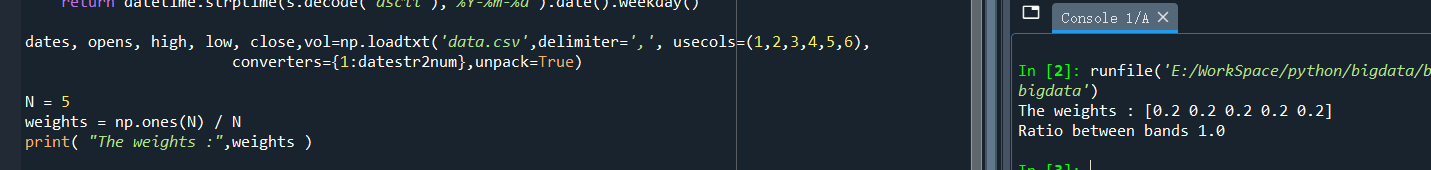
在上一篇文章中,在计算移动平均和指数平均时,计算了不同的权重,例如
[En]
In the previous article, when calculating moving averages and exponential averages, different weights were calculated, such as

和
相关权重是根据不同的计算方法计算出来的,股价可以用之前股价的线性组合来表示,即股价等于之前股价乘以各自系数的结果,但这些系数需要我们确定,也就是线性相关的权重。
[En]
The relevant weights are calculated according to different calculation methods, and a stock price can be expressed by a linear combination of the previous stock price, that is, the stock price is equal to the result of multiplying the previous stock price by their respective coefficients, but, these coefficients need us to determine, that is, a linearly related weight.
一、用线性模型预测价格
创建步骤如下:
1)先获取一个包含N个收盘价的向量(数组):
N=10
#N=len(close)
new_close = close[-N:]
new_closes= new_close[::-1]
print (new_closes)
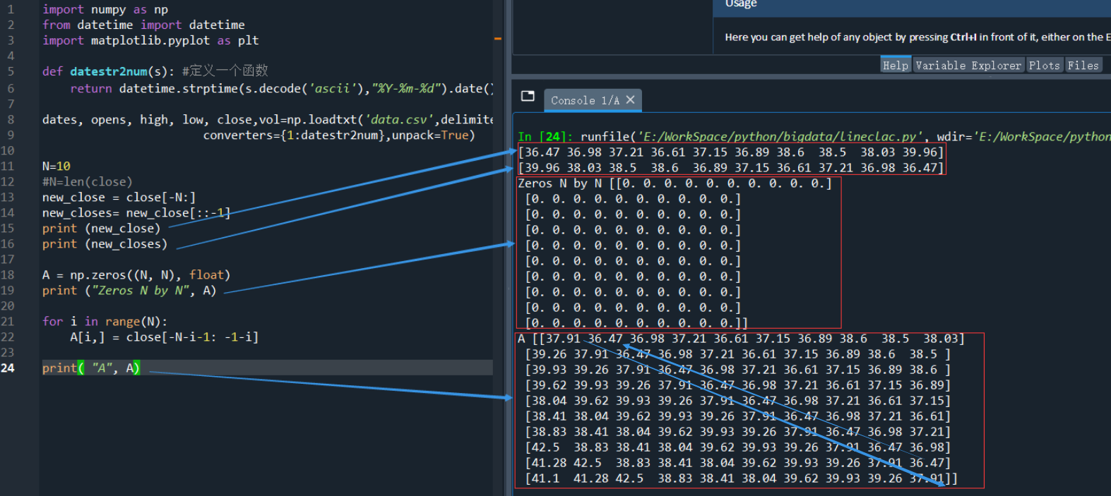
运行结果:[39.96 38.03 38.5 38.6 36.89 37.15 36.61 37.21 36.98 36.47]2)初始化一个N×N的二维数组 A ,元素全部为 0
A = np.zeros((N, N), float)
print ("Zeros N by N", A)
undefined
3)用数组new_closes的股价填充数组A
for i in range(N):
    A[i,] = close[-N-i-1: -1-i]
print( "A", A)
试一下运行结果,并观察填充后的数组A
4)选取合适的权重
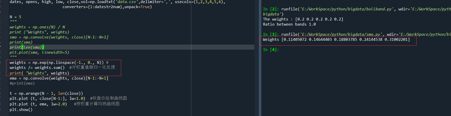
Weights [0.11405072 0.14644403 0.18803785 0.24144538 0.31002201]和The weights : [0.2 0.2 0.2 0.2 0.2]哪一种权重更合理?用线性代数的术语来说,就是解一个最小二乘法的问题。
要确定线性模型中的权重系数,就是解决最小平方和的问题,可以使用 linalg包中的 lstsq 函数来完成这个任务
(x, residuals, rank, s) = np.linalg.lstsq(A,new_closes)
其中,x是由A,new_closes通过np.linalg.lstsq()函数,即生成的权重(向量),residuals为残差数组、rank为A的秩、s为A的奇异值。
5)预测股价,用NumPy中的 dot()函数计算系数向量与最近N个价格构成的向量的点积(dot product),这个点积就是向量new_closes中价格的线性组合,系数由向量 x 提供
print( np.dot(new_closes, x))
完整代码如下:
import numpy as np
from datetime import datetime
import matplotlib.pyplot as plt

def datestr2num(s): #定义一个函数
    return datetime.strptime(s.decode('ascii'),"%Y-%m-%d").date().weekday()

dates, opens, high, low, close,vol=np.loadtxt('data.csv',delimiter=',', usecols=(1,2,3,4,5,6),
                       converters={1:datestr2num},unpack=True)

N=10
#N=len(close)
new_close = close[-N:]
new_closes= new_close[::-1]

A = np.zeros((N, N), float)

for i in range(N):
    A[i,] = close[-N-i-1: -1-i]

print( "A", A)

(x, residuals, rank, s) = np.linalg.lstsq(A,new_closes)
print(x) #权重系数向量

print('\n')
print(residuals)  #残差数组
print('\n')
print(rank) #A的秩
print(s)
print('\n')#奇异值
print( np.dot(new_closes, x))
运行结果如下:
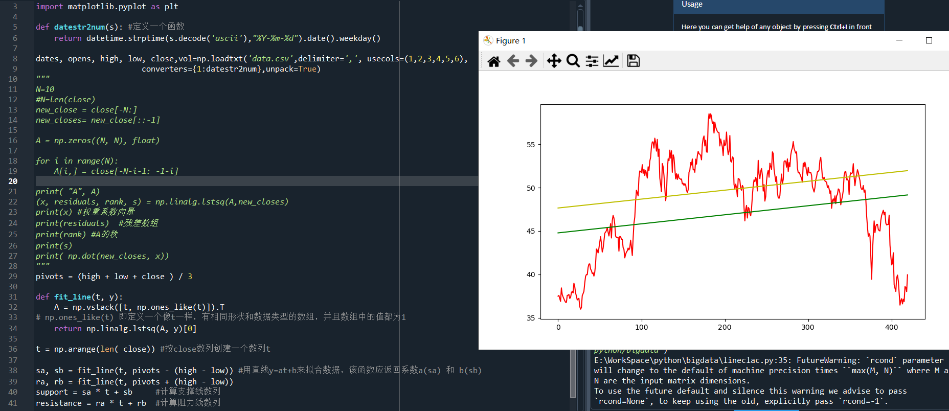
二、趋势线
趋势线是根据股价图表上许多所谓的轴心点绘制的曲线。描述价格变化的趋势。你可以让电脑以一种非常简单的方式画出趋势线。
[En]
The trend line is a curve drawn according to many so-called pivot points on the stock price chart. Describe the trend of price changes. You can let the computer draw the trend line in a very easy way.
(1) 确定枢轴点的位置。假定枢轴点位置 为最高价、最低价和收盘价的算术平均值。pivots = (high + low + close ) / 3
从支点出发,可以推算出股价的所谓阻力位和支撑位。阻力位是指股价上涨时遇到的阻力,下跌前的最高价;支撑位是指股价下跌时的最低价,反弹前的最低价(阻力位和支撑位不是客观的,它们只是一个估计值)。基于这些估计值,可以画出阻力位和支撑位的趋势线。我们将当天的价格范围定义为最高价格和最低价格之间的差额。
[En]
Starting from the pivot point, the so-called resistance level and support level of stock price can be deduced. The resistance level refers to the resistance encountered when the stock price rises and the highest price before the fall; the support level refers to the lowest price when the stock price falls and the lowest price before the rebound (resistance level and support level are not objective, they are just an estimator). Based on these estimators, the trend lines of resistance level and support level can be drawn. We define the price range of the day as the difference between the highest price and the lowest price.
(2) 定义一个函数用直线 y= at + b 来拟合数据,该函数应返回系数 a 和 b,再次用到 linalg 包中的 lstsq 函数。将直线方程重写为 y = Ax 的形式,其中 A = [t 1] , x = [a b] 。使用 ones_like 和 vstack 函数来构造数组 A
numpy.ones_like(a, dtype=None, order=’K’, subok=True) 返回与指定数组具有相同形状和数据类型的数组,并且数组中的值都为1。
numpy.vstack(tup) [source] 垂直(行)按顺序堆叠数组。 这等效于形状(N,)的1-D数组已重塑为(1,N)后沿第一轴进行concatenation。 重建除以vsplit的数组。如下两小例:
>>> a = np.array([1, 2, 3]) >>> b = np.array([2, 3, 4]) >>> np.vstack((a,b)) array([[1, 2, 3], [2, 3, 4]])
>>> a = np.array([[1], [2], [3]])
>>> b = np.array([[2], [3], [4]])
>>> np.vstack((a,b))
array([[1],
       [2],
       [3],
       [2],
       [3],
       [4]])
完整代码如下:
import numpy as np
from datetime import datetime
import matplotlib.pyplot as plt

def datestr2num(s): #定义一个函数
    return datetime.strptime(s.decode('ascii'),"%Y-%m-%d").date().weekday()

dates, opens, high, low, close,vol=np.loadtxt('data.csv',delimiter=',', usecols=(1,2,3,4,5,6),
                       converters={1:datestr2num},unpack=True)
"""
N=10
#N=len(close)
new_close = close[-N:]
new_closes= new_close[::-1]

A = np.zeros((N, N), float)

for i in range(N):
    A[i,] = close[-N-i-1: -1-i]

print( "A", A)
(x, residuals, rank, s) = np.linalg.lstsq(A,new_closes)
print(x) #权重系数向量
print(residuals)  #残差数组
print(rank) #A的秩
print(s)
print( np.dot(new_closes, x))
"""
pivots = (high + low + close ) / 3

def fit_line(t, y):
    A = np.vstack([t, np.ones_like(t)]).T
np.ones_like(t) 即定义一个像t一样,有相同形状和数据类型的数组,并且数组中的值都为1
    return np.linalg.lstsq(A, y)[0]

t = np.arange(len( close)) #按close数列创建一个数列t

sa, sb = fit_line(t, pivots - (high - low)) #用直线y=at+b来拟合数据,该函数应返回系数a(sa) 和 b(sb)
ra, rb = fit_line(t, pivots + (high - low))
support = sa * t + sb     #计算支撑线数列
resistance = ra * t + rb  #计算阻力线数列

condition = (close > support) & (close < resistance)#设置一个判断数据点是否位于趋势线之间的条件,作为 where 函数的参数
between_bands = np.where(condition)

plt.plot(t, close,color='r')
plt.plot(t, support,color='g')
plt.plot(t, resistance,color='y')
plt.show()
运行结果:
三、数组的修剪和压缩
NumPy中的 ndarray 类定义了许多方法,可以对象上直接调用。通常情况下,这些方法会返回一个数组。
ndarray 对象的方法相当多,像前面遇到的 var 、 sum 、 std 、 argmax 、argmin 以及 mean 函数也均为 ndarray 方法。下面介绍一下数组的修前与压缩。
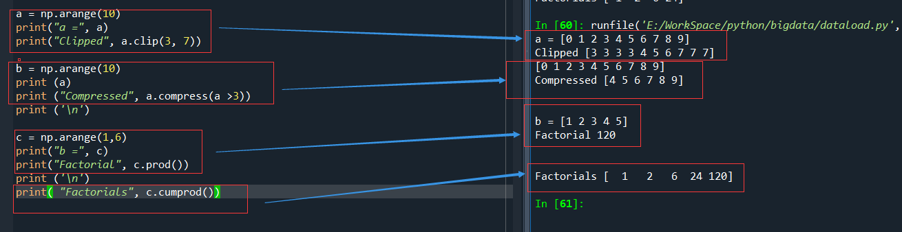
1、 clip 方法返回一个修剪过的数组:将所有比给定最大值还大的元素全部设为给定的最大值,而所有比给定最小值还小的元素全部设为给定的最小值
a = np.arange(10)
print("a =", a)
print("Clipped", a.clip(3, 7))
运行结果:
a = [0 1 2 3 4 5 6 7 8 9]
Clipped [3 3 3 3 4 5 6 7 7 7]
很明显,a.clip(3,7)将数组a中的小于3的设置为3,大于7的全部设置为7.
2、 compress 方法返回一个根据给定条件筛选后的数组
b = np.arange(10)
print (a)
print ("Compressed", a.compress(a >3))
运行结果:
[0 1 2 3 4 5 6 7 8 9]
Compressed [4 5 6 7 8 9]
四、阶乘
prod() 方法,可以计算数组中所有元素的乘积.
c = np.arange(1,5)
print("b =", c)
print("Factorial", c.prod())
运行结果:
b = [1 2 3 4]
Factorial 24
如果想知道1~8的所有阶乘值,调用 cumprod()方法,计算数组元素的累积乘积。
print( "Factorials", c.cumprod())
运行结果:
Factorials [ 1 2 6 24 120]
本篇主要介绍了一个通过现在有数据,用函数 y= at + b 来拟合数据进行线性拟合后,用 linalg包中的 lstsq 函数来完成最小二乘相关后,预测股价的实例,来了解了一些numpy的函数及作用;同时介绍 了数据修剪及压缩和阶乘的计算。
Original: https://www.cnblogs.com/codingchen/p/16304038.html
Author: PursuitingPeak
Title: Python数据分析–Numpy常用函数介绍(4)–Numpy中的线性关系和数据修剪压缩
原创文章受到原创版权保护。转载请注明出处:https://www.johngo689.com/499501/
转载文章受原作者版权保护。转载请注明原作者出处!