

激活函数学习(2022.2.28)
- 所用软件及环境(Matlab+PyCharm+Python+Tensorflow+Keras+PyTorch)
- 1、激活函数简介
* - 1.1 Activation Function
- 1.2 PyTorch激活函数API
- 1.3 TensorFlow + Keras激活函数API
- 2、常用的激活函数(公式+曲线图)
* - 2.1 线性激活函数
– - 2.2 非线性激活函数
– - 2.3 tensorflow.keras调用激活函数示例
- 2.4 PyTorch调用激活函数示例
- 3 Matlab代码绘制各激活函数曲线图
* - 3.1 Matlab各激活函数定义
- 3.2 Matlab各激活函数分别绘制(多个图)
- 3.3 Matlab绘制各激活函数一张图
- 4、Python代码绘制各函数曲线图
* - 4.1 Python各激活函数分别绘制(多个图)
- 4.2 Python绘制各激活函数一张图
所用软件及环境(Matlab+PyCharm+Python+Tensorflow+Keras+PyTorch)


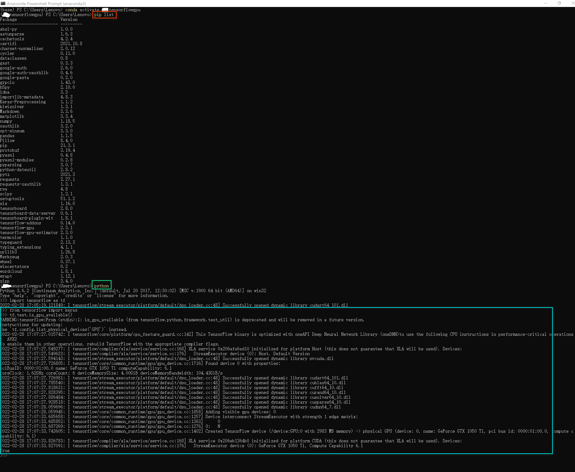
Python + TensorFlow + Keras
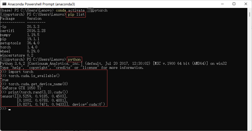
Python+PyTorch
; 1、激活函数简介
1.1 Activation Function
Activation Function( 激活函数)就是一个从 x到 y的映射函数 y=f(x),它主要应用在深度学习和神经网络中的神经元,负责将输入 Input通过函数作用后映射到输出 Output。
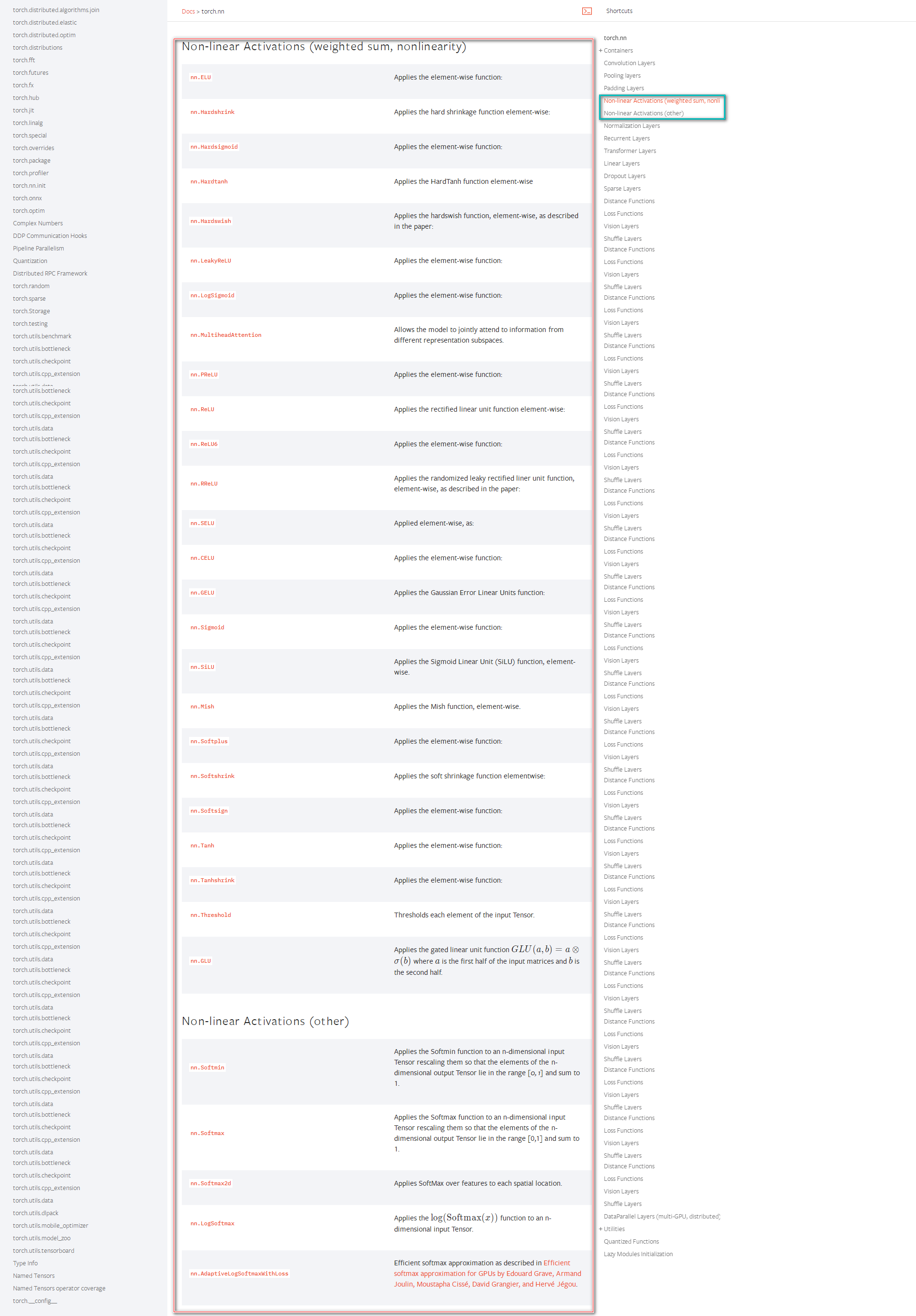
1.2 PyTorch激活函数API
PyTorch官网上 API文档可以看到torch.nn和torch.nn.functional都介绍到所用的激活函数,包含nn.Softmin、 nn.Softmax、nn.Softmax2d、nn.LogSoftmax、nn.AdaptiveLogSoftmaxWithLoss、nn.GLU、nn.Threshold、nn.Tanhshrink、nn.Tanh、nn.Softsign、nn.Softshrink、nn.Softplus、nn.Mish、nn.SiLU、nn.Sigmoid、nn.GELU、nn.CELU、nn.SELU、nn.RReLU、nn.ReLU6、nn.ReLU、nn.PReLU、nn.MultiheadAttention、nn.LogSigmoid、nn.LeakyReLU、nn.Hardswish、nn.Hardswish、nn.Hardtanh、nn.Hardsigmoid、nn.Hardshrink、nn.ELU等。

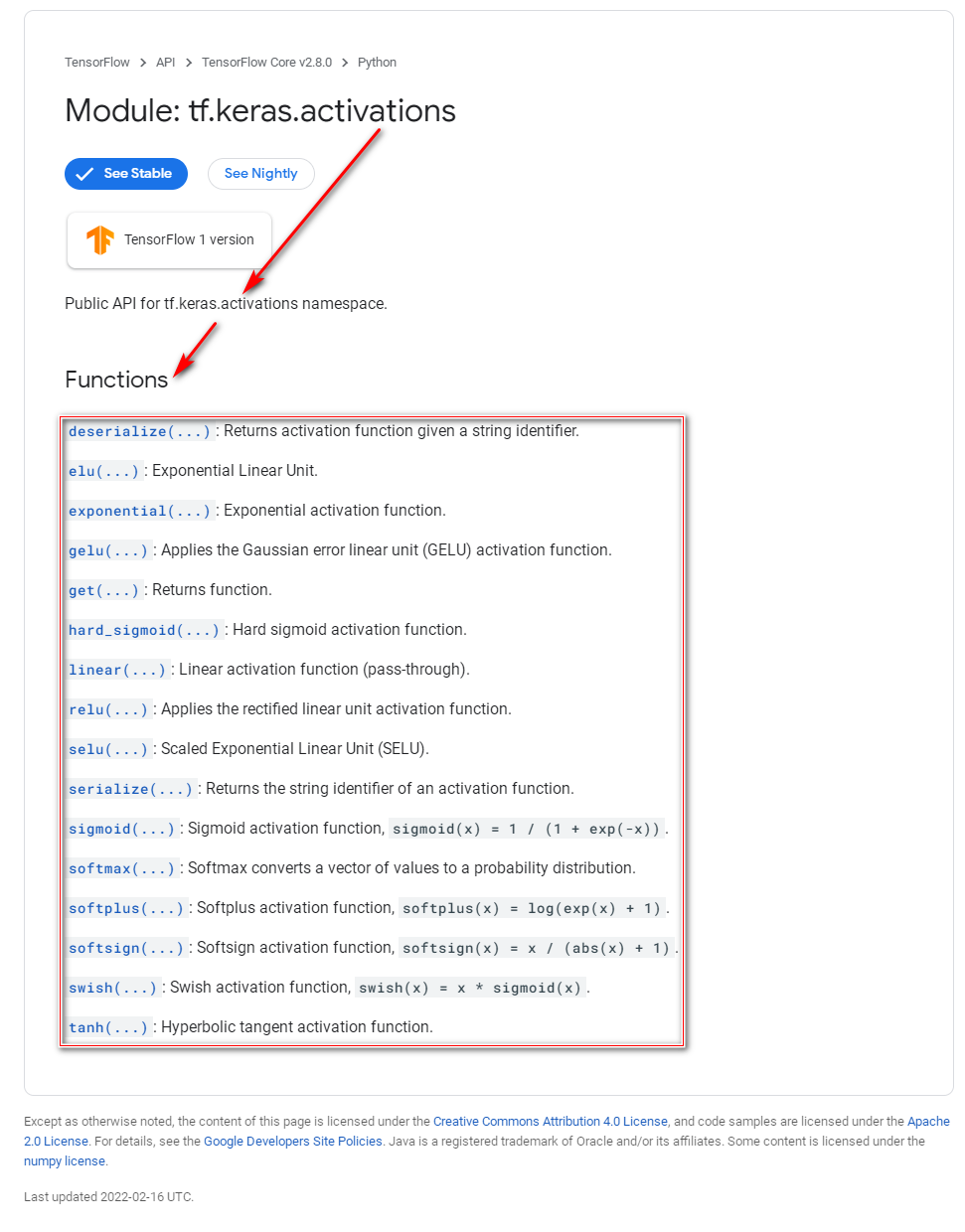
; 1.3 TensorFlow + Keras激活函数API
Keras官网tf.keras.activations和 TensorFlow官网tf.keras.activations的 API文档介绍其所用到的激活函数有:relu、sigmoid、softmax、softplus、softsign、tanh、selu、elu、exponential,deserialize、elu、exponential、gelu、get、hard_sigmoid、linear、reluseluserializesigmoidsoftmax、softplus、softsign、swish、tanh等。

; 2、常用的激活函数(公式+曲线图)
2.1 线性激活函数
2.1.1 Linear

y = x y=x y =x

import tensorflow as tf
a = tf.constant([-3.0,-1.0, 0.0,1.0,3.0], dtype = tf.float32)
b = tf.keras.activations.linear(a)
print(b)
运行结果:
tf.Tensor([-3. -1. 0. 1. 3.], shape=(5,), dtype=float32)
2.2 非线性激活函数
与线性激励函数不同,非线性激励函数的引入可以增加神经网络的非线性,而不仅仅是简单的线性矩阵乘法。
[En]
Different from the linear activation function, the introduction of the nonlinear activation function can increase the nonlinearity of the neural network, which is not just a simple linear matrix multiplication.
2.2.1 Exponential

e x p o n e n t i a l ( x ) = e x exponential(x) = e^{x}e x p o n e n t i a l (x )=e x

import tensorflow as tf
a = tf.constant([-3.0,-1.0, 0.0,1.0,3.0], dtype = tf.float32)
b = tf.keras.activations.exponential(a)
print(b)
运行结果:
tf.Tensor([ 0.04978707 0.36787945 1. 2.7182817 20.085537 ], shape=(5,), dtype=float32)
2.2.2 Hard_sigmoid
H a r d ‾ s i g m o i d ( x ) = { 0 x < − 2.5 0.2 x + 0.5 − 2.5 ≤ x ≤ 2.5 1 x > 2.5 Hard\underline{~~}sigmoid(x)=\begin{cases} 0 & x H a r d s i g m o i d (x )=⎩⎪⎨⎪⎧0 0 .2 x +0 .5 1 x <−2 .5 −2 .5 ≤x ≤2 .5 x >2 .5

import tensorflow as tf
a = tf.constant([-3.0,-1.0, 0.0,1.0,3.0], dtype = tf.float32)
b = tf.keras.activations.hard_sigmoid(a)
print(b)
运行结果:
tf.Tensor([0. 0.3 0.5 0.7 1. ], shape=(5,), dtype=float32)
2.2.3 Sigmoid

S i g m o i d ( x ) = 1 1 + e − x Sigmoid(x) = \frac{1}{1+e^{-x}}S i g m o i d (x )=1 +e −x 1

import tensorflow as tf
print('sigmoid(x) = 1 / (1 + exp(-x))')
a = tf.constant([-20, -1.0, 0.0, 1.0, 20], dtype = tf.float32)
b = tf.keras.activations.sigmoid(a).numpy()
print(b)
运行结果:
sigmoid(x) = 1 / (1 + exp(-x))
[2.0611535e-09 2.6894143e-01 5.0000000e-01 7.3105860e-01 1.0000000e+00]
2.2.4 Swish

S w i s h ( x ) = x ⋅ S i g m o i d ( x ) = x 1 + e − x Swish(x) = x\cdot Sigmoid(x) = \frac{x}{1+e^{-x}}S w i s h (x )=x ⋅S i g m o i d (x )=1 +e −x x

import tensorflow as tf
a = tf.constant([-20, -1.0, 0.0, 1.0, 20], dtype = tf.float32)
b = tf.keras.activations.swish(a)
print(b)
运行结果:
tf.Tensor([-4.1223068e-08 -2.6894143e-01 0.0000000e+00 7.3105860e-01 2.0000000e+01], shape=(5,), dtype=float32)
2.2.5 Tanh
Hyperbolic tangent activation function

T a n h ( x ) = e x − e − x e x + e − x Tanh(x) = \frac{e^{x}-e^{-x}}{e^{x}+e^{-x}}T a n h (x )=e x +e −x e x −e −x

import tensorflow as tf
a = tf.constant([-3.0,-1.0, 0.0,1.0,3.0], dtype = tf.float32)
b = tf.keras.activations.tanh(a)
print(b)
运行结果:
tf.Tensor([-0.9950548 -0.7615942 0. 0.7615942 0.9950548], shape=(5,), dtype=float32)
2.2.6 Softmax
Softmax converts a vector of values to a probability distribution.

S o f t m a x ( x i ) = e x i ∑ j = 1 n e x j Softmax(x_{i}) = \frac{e^{x_i}}{\sum_{j=1}^n e^{x_j}}S o f t m a x (x i )=∑j =1 n e x j e x i S o f t m a x ( x ⃗ ) = [ S o f t m a x ( x 1 ) , . . . , S o f t m a x ( x i ) , . . . , S o f t m a x ( x n ) ] T Softmax(\vec{x}) =[Softmax(x_{1}),…,Softmax(x_{i}),…,Softmax(x_{n})]^{T}S o f t m a x (x )=[S o f t m a x (x 1 ),…,S o f t m a x (x i ),…,S o f t m a x (x n )]T

import tensorflow as tf
inputs = tf.random.normal(shape=(3,4))
print(inputs)
outputs = tf.keras.activations.softmax(inputs)
print(outputs)
print(tf.reduce_sum(outputs[0,:]))
运行结果:
tf.Tensor([[-1.4463423  -1.2136649   0.37711483 -1.5163935 ]
 [ 1.1458701   0.69421154  0.5825411  -0.6992794 ]
 [ 0.90473056  0.9367949   0.5104403   0.40904504]], shape=(3, 4), dtype=float32)
tf.Tensor([[0.10652403 0.13443059 0.6597281  0.09931726]
 [0.4230326  0.26929048 0.240837   0.06683987]
 [0.3015777  0.31140423 0.20331109 0.183707  ]], shape=(3, 4), dtype=float32)
tf.Tensor(1.0, shape=(), dtype=float32)
import tensorflow as tf
x = tf.constant([-3.0, -1.0, 0.0, 2.0], dtype = tf.float32)
layer = tf.keras.layers.Softmax()
output = layer(x)
list(output.numpy())
print(tf.reduce_sum(output))
运行结果:
[0.0056533027, 0.041772567, 0.11354961, 0.8390245]
tf.Tensor(0.99999994, shape=(), dtype=float32)
2.2.7 Softplus

S o f t p l u s ( x ) = l o g ( e x + 1 ) Softplus(x) = log(e^{x}+1)S o f t p l u s (x )=l o g (e x +1 )

import tensorflow as tf
a = tf.constant([-20, -1.0, 0.0, 1.0, 20], dtype = tf.float32)
b = tf.keras.activations.softplus(a)
print(b)
运行结果:
tf.Tensor([2.0611535e-09 3.1326169e-01 6.9314718e-01 1.3132616e+00 2.0000000e+01], shape=(5,), dtype=float32)
2.2.8 Softsign

S o f t s i g n ( x ) = x 1 + ∣ x ∣ Softsign(x) = \frac{x}{1+|x|}S o f t s i g n (x )=1 +∣x ∣x

import tensorflow as tf
a = tf.constant([-1.0, 0.0, 1.0], dtype=tf.float32)
b = tf.keras.activations.softsign(a)
print(b)
运行结果:
tf.Tensor([-0.5 0. 0.5], shape=(3,), dtype=float32)
2.2.9 eLU
The exponential linear unit (ELU) activation function:
alpha: Scale for the negative factor.

e L U ( x ) = { x x ≥ 0 α ⋅ ( e x − 1 ) x < 0 ( α > 0 ) eLU(x)=\begin{cases} x & x≥0 \ \alpha \cdot (e^{x}-1)& x e L U (x )={x α⋅(e x −1 )x ≥0 x <0 (α>0 )

import tensorflow as tf
a = tf.constant([-4.0,-2.0, 0.0,2.0,4.0], dtype = tf.float32)
b = tf.keras.activations.elu(a)
print(b)
运行结果:
tf.Tensor([-0.9816844 -0.86466473 0. 2. 4.], shape=(5,), dtype=float32)
import tensorflow as tf
x = tf.constant([-3.0, -1.0, 0.0, 2.0], dtype = tf.float32)
layer = tf.keras.layers.ELU()
output = layer(x)
list(output.numpy())
x = tf.constant([-3.0, -1.0, 0.0, 2.0], dtype = tf.float32)
layer = tf.keras.layers.ELU(alpha = 1.5)
output = layer(x)
list(output.numpy())
运行结果:
[-0.95021296, -0.63212055, 0.0, 2.0]
[-1.4253194, -0.9481808, 0.0, 2.0]
2.2.10 GeLU
the Gaussian error linear unit (GELU) activation function
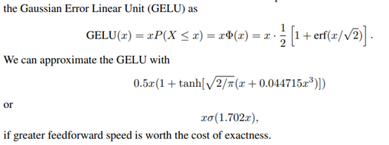

G e L U ( x ) = x ⋅ Φ ( x ) = x 2 [ 1 + e r f ( x 2 ) ] GeLU(x) = x\cdotΦ(x) = \frac{x}{2}[1+erf(\frac{x}{\sqrt{2}})]G e L U (x )=x ⋅Φ(x )=2 x [1 +e r f (2 x )]
G e L U ( x ) = x ⋅ Φ ( x ) = x 2 ( 1 + t a n h [ 2 π ( x + 0.044715 x 3 ) ] ) GeLU(x) = x\cdotΦ(x) = \frac{x}{2}(1+tanh[\frac{2}{\sqrt{\pi}}(x+0.044715x^{3})])G e L U (x )=x ⋅Φ(x )=2 x (1 +t a n h [π2 (x +0 .0 4 4 7 1 5 x 3 )])
The gaussian error linear activation: 0.5 * x * (1 + tanh(sqrt(2 / pi) * (x + 0.044715 * x^3))) if approximate is True or x * P(X
Original: https://blog.csdn.net/jing_zhong/article/details/123160553
Author: jing_zhong
Title: 激活函数学习(2022.2.28)
原创文章受到原创版权保护。转载请注明出处:https://www.johngo689.com/497606/
转载文章受原作者版权保护。转载请注明原作者出处!