

目录
经典的图像分类模型
AlexNet
学习目标
- 知道AlexNet网络结构
- 能够利用AlexNet完成图像分类
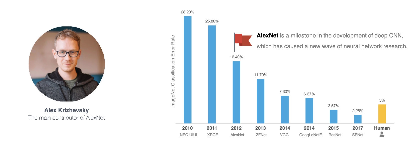

2012年,AlexNet横空出世,该模型的名字源于论文第一作者的姓名Alex Krizhevsky 。AlexNet使用了8层卷积神经网络,以很大的优势赢得了ImageNet 2012图像识别挑战赛。它首次证明了学习到的特征可以超越手工设计的特征,从而一举打破计算机视觉研究的方向。
; AlexNet的网络架构
AlexNet与LeNet的设计理念非常相似,但也有显著的区别,其网络架构如下图所示:
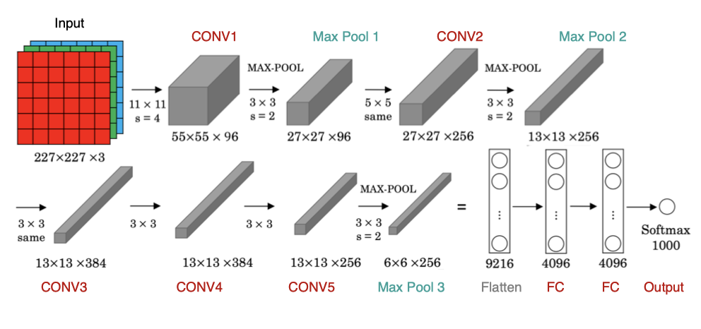
该网络的特点是:
- AlexNet包含8层变换,有5层卷积和2层全连接隐藏层,以及1个全连接输出层
- AlexNet第一层中的卷积核形状是11×1111×11。第二层中的卷积核形状减小到5×55×5,之后全采用3×33×3。所有的池化层窗口大小为3×33×3、步幅为2的最大池化。
- AlexNet将sigmoid激活函数改成了ReLU激活函数,使计算更简单,网络更容易训练
- AlexNet通过dropOut来控制全连接层的模型复杂度。
- AlexNet引入了大量的图像增强,如翻转、裁剪和颜色变化,从而进一步扩大数据集来缓解过拟合。
在tf.keras中实现AlexNet模型:
net = tf.keras.models.Sequential([

    tf.keras.layers.Conv2D(filters=96,kernel_size=11,strides=4,activation='relu'),

    tf.keras.layers.MaxPool2D(pool_size=3, strides=2),

    tf.keras.layers.Conv2D(filters=256,kernel_size=5,padding='same',activation='relu'),

    tf.keras.layers.MaxPool2D(pool_size=3, strides=2),

    tf.keras.layers.Conv2D(filters=384,kernel_size=3,padding='same',activation='relu'),

    tf.keras.layers.Conv2D(filters=384,kernel_size=3,padding='same',activation='relu'),

    tf.keras.layers.Conv2D(filters=256,kernel_size=3,padding='same',activation='relu'),

    tf.keras.layers.MaxPool2D(pool_size=3, strides=2),

    tf.keras.layers.Flatten(),

    tf.keras.layers.Dense(4096,activation='relu'),

    tf.keras.layers.Dropout(0.5),

    tf.keras.layers.Dense(4096,activation='relu'),

    tf.keras.layers.Dropout(0.5),

    tf.keras.layers.Dense(10,activation='softmax')
])
我们构造一个高和宽均为227的单通道数据样本来看一下模型的架构:
X = tf.random.uniform((1,227,227,1)
y = net(X)

net.summay()
网络架构如下:
Model: "sequential"
_________________________________________________________________
Layer (type)                 Output Shape              Param
=================================================================
conv2d (Conv2D)              (1, 55, 55, 96)           11712
_________________________________________________________________
max_pooling2d (MaxPooling2D) (1, 27, 27, 96)           0
_________________________________________________________________
conv2d_1 (Conv2D)            (1, 27, 27, 256)          614656
_________________________________________________________________
max_pooling2d_1 (MaxPooling2 (1, 13, 13, 256)          0
_________________________________________________________________
conv2d_2 (Conv2D)            (1, 13, 13, 384)          885120
_________________________________________________________________
conv2d_3 (Conv2D)            (1, 13, 13, 384)          1327488
_________________________________________________________________
conv2d_4 (Conv2D)            (1, 13, 13, 256)          884992
_________________________________________________________________
max_pooling2d_2 (MaxPooling2 (1, 6, 6, 256)            0
_________________________________________________________________
flatten (Flatten)            (1, 9216)                 0
_________________________________________________________________
dense (Dense)                (1, 4096)                 37752832
_________________________________________________________________
dropout (Dropout)            (1, 4096)                 0
_________________________________________________________________
dense_1 (Dense)              (1, 4096)                 16781312
_________________________________________________________________
dropout_1 (Dropout)          (1, 4096)                 0
_________________________________________________________________
dense_2 (Dense)              (1, 10)                   40970
=================================================================
Total params: 58,299,082
Trainable params: 58,299,082
Non-trainable params: 0
_________________________________________________________________
手写数字势识别
AlexNet使用ImageNet数据集进行训练,但因为ImageNet数据集较大训练时间较长,我们仍用前面的MNIST数据集来演示AlexNet。读取数据的时将图像高和宽扩大到AlexNet使用的图像高和宽227。这个通过 tf.image.resize_with_pad来实现。
数据读取
import numpy as np

(train_images, train_labels), (test_images, test_labels) = mnist.load_data()

train_images = np.reshape(train_images,(train_images.shape[0],train_images.shape[1],train_images.shape[2],1))

test_images = np.reshape(test_images,(test_images.shape[0],test_images.shape[1],test_images.shape[2],1))
由于使用所有数据进行训练需要较长的时间,因此我们定义了两种方法来获取部分数据,并将图像调整为2270227进行模型训练:
[En]
Because it takes a long time to train with all the data, we define two methods to obtain some of the data, and adjust the image to 2270227 for model training:
def get_train(size):

    index = np.random.randint(0, np.shape(train_images)[0], size)

    resized_images = tf.image.resize_with_pad(train_images[index],227,227,)

    return resized_images.numpy(), train_labels[index]

def get_test(size):

    index = np.random.randint(0, np.shape(test_images)[0], size)

    resized_images = tf.image.resize_with_pad(test_images[index],227,227,)

    return resized_images.numpy(), test_labels[index]
调用上述两种方法,获取参与模型训练和测试的数据集:
[En]
Call the above two methods to get the datasets that participate in model training and testing:
train_images,train_labels = get_train(256)
test_images,test_labels = get_test(128)
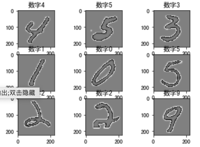
为了让您更好地了解,我们展示了以下数据:
[En]
In order for you to understand better, we show the data:
for i in range(9):
    plt.subplot(3,3,i+1)

    plt.imshow(train_images[i].astype(np.int8).squeeze(), cmap='gray', interpolation='none')

    plt.title("数字{}".format(train_labels[i]))
结果为:
我们使用上面创建的模型进行培训和评估。
[En]
We use the model created above for training and evaluation.
模型编译
optimizer = tf.keras.optimizers.SGD(learning_rate=0.01, momentum=0.0, nesterov=False)

net.compile(optimizer=optimizer,
              loss='sparse_categorical_crossentropy',
              metrics=['accuracy'])
模型训练
net.fit(train_images,train_labels,batch_size=128,epochs=3,verbose=1,validation_split=0.1)
训练输出为:
Epoch 1/3
2/2 [==============================] - 3s 2s/step - loss: 2.3003 - accuracy: 0.0913 - val_loss: 2.3026 - val_accuracy: 0.0000e+00
Epoch 2/3
2/2 [==============================] - 3s 2s/step - loss: 2.3069 - accuracy: 0.0957 - val_loss: 2.3026 - val_accuracy: 0.0000e+00
Epoch 3/3
2/2 [==============================] - 4s 2s/step - loss: 2.3117 - accuracy: 0.0826 - val_loss: 2.3026 - val_accuracy: 0.0000e+00
模型评估
net.evaluate(test_images,test_labels,verbose=1)
输出为:
4/4 [==============================] - 1s 168ms/step - loss: 2.3026 - accuracy: 0.0781
[2.3025851249694824, 0.078125]
如果我们使用整个数据集来训练网络并评估结果:
[En]
If we use the entire dataset to train the network and evaluate the results:
[0.4866700246334076, 0.8395]
VGG
学习目标
- 知道VGG网络结构的特点
- 能够利用VGG完成图像分类
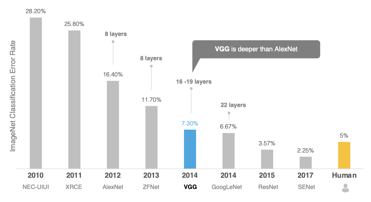
2014年,牛津大学计算机视觉组(Visual Geometry Group)和Google DeepMind公司的研究员一起研发出了新的深度卷积神经网络:VGGNet,并取得了ILSVRC2014比赛分类项目的第二名,主要贡献是使用很小的卷积核(3×3)构建卷积神经网络结构,能够取得较好的识别精度,常用来提取图像特征的VGG-16和VGG-19。
; VGG的网络架构
VGG可以看成是加深版的AlexNet,整个网络由卷积层和全连接层叠加而成,和AlexNet不同的是,VGG中使用的都是小尺寸的卷积核(3×3),其网络架构如下图所示:
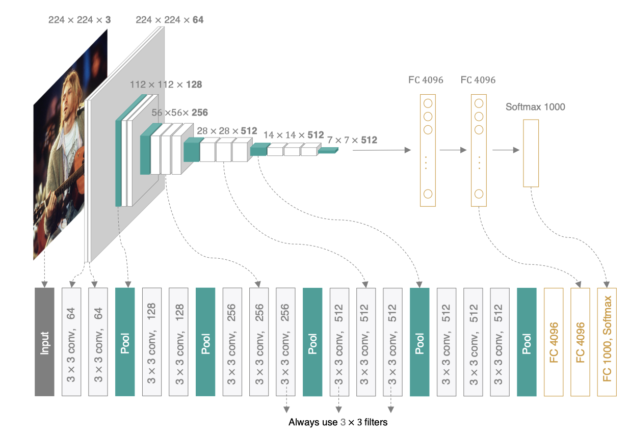
VGGNet使用的全部都是3×3的小卷积核和2×2的池化核,通过不断加深网络来提升性能。VGG可以通过重复使用简单的基础块来构建深度模型。
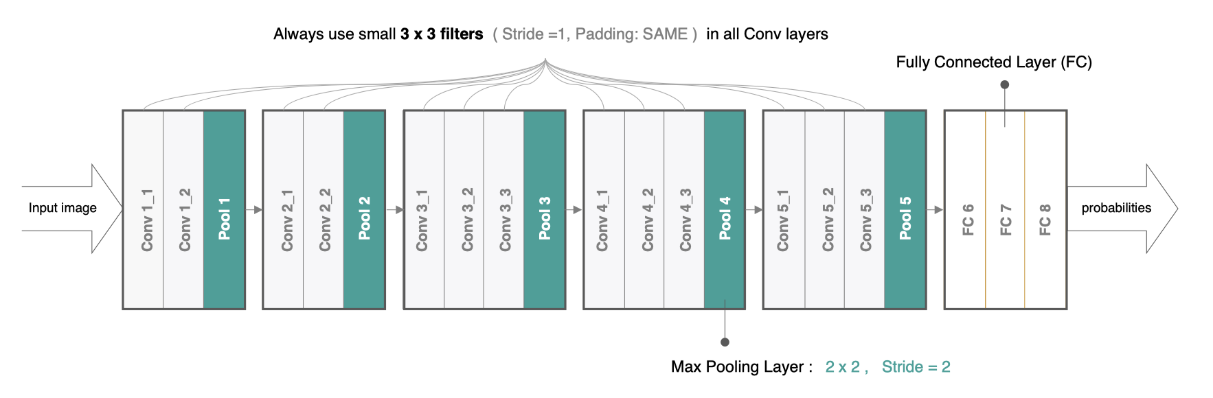
在tf.keras中实现VGG模型,首先来实现VGG块,它的组成规律是:连续使用多个相同的填充为1、卷积核大小为3×33×3的卷积层后接上一个步幅为2、窗口形状为2×22×2的最大池化层。卷积层保持输入的高和宽不变,而池化层则对其减半。我们使用 vgg_block函数来实现这个基础的VGG块,它可以指定卷积层的数量 num_convs和每层的卷积核个数num_filters:
def vgg_block(num_convs, num_filters):

    blk = tf.keras.models.Sequential()

    for _ in range(num_convs):

        blk.add(tf.keras.layers.Conv2D(num_filters,kernel_size=3,
                                    padding='same',activation='relu'))

    blk.add(tf.keras.layers.MaxPool2D(pool_size=2, strides=2))
    return blk
VGG16网络有5个卷积块,前2块使用两个卷积层,而后3块使用三个卷积层。第一块的输出通道是64,之后每次对输出通道数翻倍,直到变为512。
conv_arch = ((2, 64), (2, 128), (3, 256), (3, 512), (3, 512))
因为这个网络使用了13个卷积层和3个全连接层,所以经常被称为VGG-16,通过制定conv_arch得到模型架构后构建VGG16:
def vgg(conv_arch):

    net = tf.keras.models.Sequential()

    for (num_convs, num_filters) in conv_arch:
        net.add(vgg_block(num_convs, num_filters))

    net.add(tf.keras.models.Sequential([

        tf.keras.layers.Flatten(),

        tf.keras.layers.Dense(4096, activation='relu'),

        tf.keras.layers.Dropout(0.5),

        tf.keras.layers.Dense(4096, activation='relu'),

        tf.keras.layers.Dropout(0.5),

        tf.keras.layers.Dense(10, activation='softmax')]))
    return net

net = vgg(conv_arch)
我们构造一个高和宽均为224的单通道数据样本来看一下模型的架构:
X = tf.random.uniform((1,224,224,1))
y = net(X)

net.summay()
网络架构如下:
Model: "sequential_15"
_________________________________________________________________
Layer (type)                 Output Shape              Param
=================================================================
sequential_16 (Sequential)   (1, 112, 112, 64)         37568
_________________________________________________________________
sequential_17 (Sequential)   (1, 56, 56, 128)          221440
_________________________________________________________________
sequential_18 (Sequential)   (1, 28, 28, 256)          1475328
_________________________________________________________________
sequential_19 (Sequential)   (1, 14, 14, 512)          5899776
_________________________________________________________________
sequential_20 (Sequential)   (1, 7, 7, 512)            7079424
_________________________________________________________________
sequential_21 (Sequential)   (1, 10)                   119586826
=================================================================
Total params: 134,300,362
Trainable params: 134,300,362
Non-trainable params: 0
__________________________________________________________________
手写数字势识别
因为ImageNet数据集较大训练时间较长,我们仍用前面的MNIST数据集来演示VGGNet。读取数据的时将图像高和宽扩大到VggNet使用的图像高和宽224。这个通过 tf.image.resize_with_pad来实现。
数据读取
首先获取数据,并进行维度调整:
import numpy as np

(train_images, train_labels), (test_images, test_labels) = mnist.load_data()

train_images = np.reshape(train_images,(train_images.shape[0],train_images.shape[1],train_images.shape[2],1))

test_images = np.reshape(test_images,(test_images.shape[0],test_images.shape[1],test_images.shape[2],1))
由于使用全部数据进行训练需要较长的时间,因此我们定义了两种方法来获取部分数据,并将图像调整为224到224进行模型训练:
[En]
Because it takes a long time to train with all the data, we define two methods to obtain some of the data, and adjust the image to 224 to 224 for model training:
def get_train(size):

    index = np.random.randint(0, np.shape(train_images)[0], size)

    resized_images = tf.image.resize_with_pad(train_images[index],224,224,)

    return resized_images.numpy(), train_labels[index]

def get_test(size):

    index = np.random.randint(0, np.shape(test_images)[0], size)

    resized_images = tf.image.resize_with_pad(test_images[index],224,224,)

    return resized_images.numpy(), test_labels[index]
调用上述两种方法,获取参与模型训练和测试的数据集:
[En]
Call the above two methods to get the datasets that participate in model training and testing:
train_images,train_labels = get_train(256)
test_images,test_labels = get_test(128)
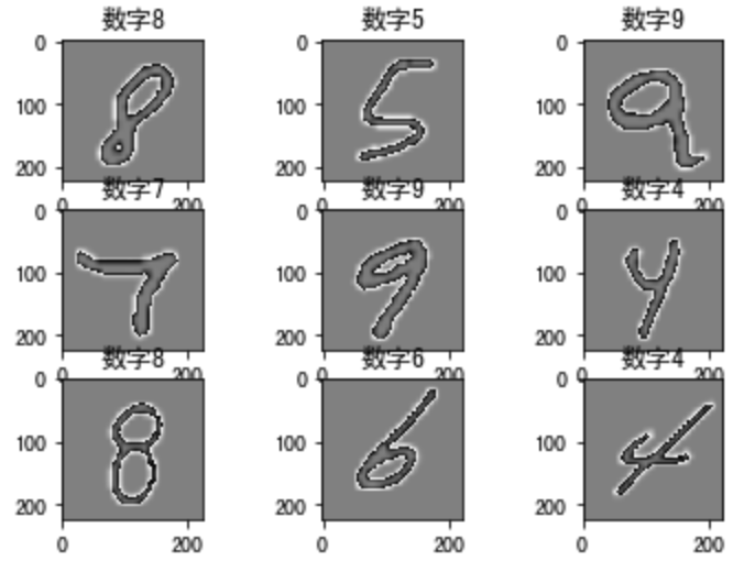
为了让您更好地了解,我们展示了以下数据:
[En]
In order for you to understand better, we show the data:
for i in range(9):
    plt.subplot(3,3,i+1)

    plt.imshow(train_images[i].astype(np.int8).squeeze(), cmap='gray', interpolation='none')

    plt.title("数字{}".format(train_labels[i]))
结果为:
我们使用上面创建的模型进行培训和评估。
[En]
We use the model created above for training and evaluation.
模型编译
optimizer = tf.keras.optimizers.SGD(learning_rate=0.01, momentum=0.0)

net.compile(optimizer=optimizer,
              loss='sparse_categorical_crossentropy',
              metrics=['accuracy'])
模型训练
net.fit(train_images,train_labels,batch_size=128,epochs=3,verbose=1,validation_split=0.1)
遇到问题: 进行模型训练时,一直遇到内核似乎挂掉了,它很快将自动重启。
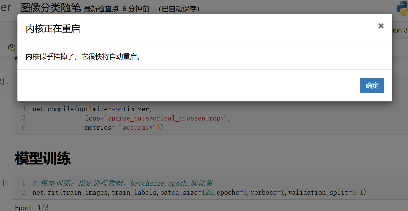
我参考一篇博客,建议卸载重新安装jupyter,然后我照做了,结果我之前安装的库都没了,都要重新安装,一个多小时白白浪费了。。。。最后还是存在这个问题,我真的是服了啊,谁这么缺德,写这样的文章,这不是害人吗????。。。。。痛苦!!!!
那么我们必须先跳过这一步。无论如何,如果我们有经验,当我们必须解决它时,我们会讨论它。我为我之前安装的库感到抱歉。如果你说不,它就会消失。
[En]
Then we have to skip this step first. Anyway, if we have experience, we’ll talk about it when we have to solve it. I feel sorry for the library I installed before. If you say no, it will be gone.
训练输出为:
Epoch 1/3
2/2 [==============================] - 34s 17s/step - loss: 2.6026 - accuracy: 0.0957 - val_loss: 2.2982 - val_accuracy: 0.0385
Epoch 2/3
2/2 [==============================] - 27s 14s/step - loss: 2.2604 - accuracy: 0.1087 - val_loss: 2.4905 - val_accuracy: 0.1923
Epoch 3/3
2/2 [==============================] - 29s 14s/step - loss: 2.3650 - accuracy: 0.1000 - val_loss: 2.2994 - val_accuracy: 0.1538
模型评估
net.evaluate(test_images,test_labels,verbose=1)
输出为:
4/4 [==============================] - 5s 1s/step - loss: 2.2955 - accuracy: 0.1016
[2.2955007553100586, 0.1015625]
如果我们使用整个数据集来训练网络并评估结果:
[En]
If we use the entire dataset to train the network and evaluate the results:
[0.31822608125209806, 0.8855]
GoogLeNet
学习目标
- 知道GoogLeNet网络结构的特点
- 能够利用GoogLeNet完成图像分类
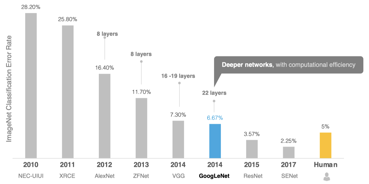
GoogLeNet的名字不是GoogleNet,而是GoogLeNet,这是为了致敬LeNet。GoogLeNet和AlexNet/VGGNet这类依靠加深网络结构的深度的思想不完全一样。GoogLeNet在加深度的同时做了结构上的创新,引入了一个叫做Inception的结构来代替之前的卷积加激活的经典组件。GoogLeNet在ImageNet分类比赛上的Top-5错误率降低到了6.7%。
; Inception 块
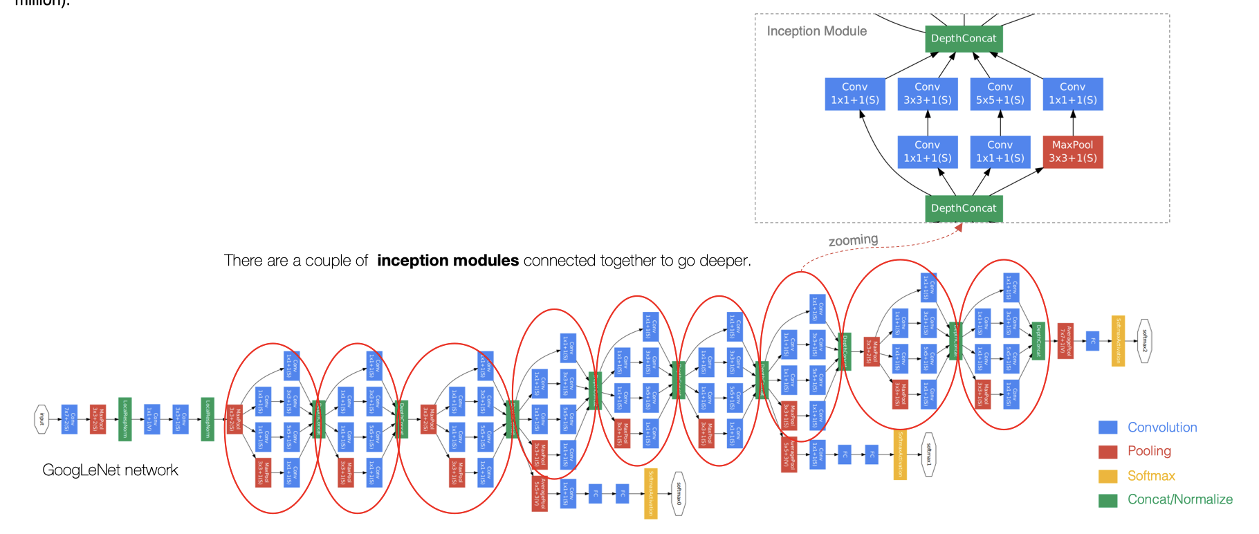
GoogLeNet中的基础卷积块叫作Inception块,得名于同名电影《盗梦空间》(Inception)。Inception块在结构比较复杂,如下图所示:
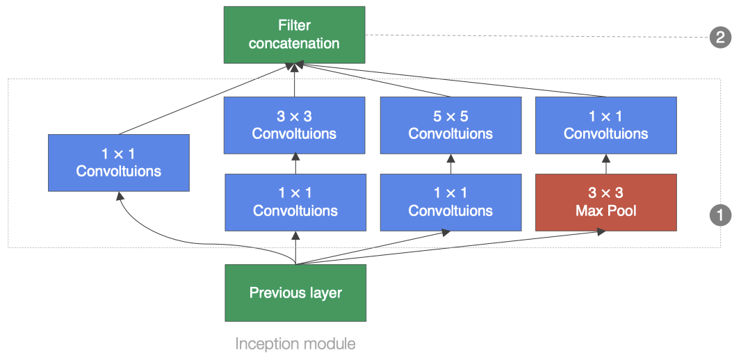
Inception块里有4条并行的线路。前3条线路使用窗口大小分别是1×11×1、3×33×3和5×55×5的卷积层来抽取不同空间尺寸下的信息,其中中间2个线路会对输入先做1×11×1卷积来减少输入通道数,以降低模型复杂度。第4条线路则使用3×33×3最大池化层,后接1×11×1卷积层来改变通道数。4条线路都使用了合适的填充来使输入与输出的高和宽一致。最后我们将每条线路的输出在通道维上连结,并向后进行传输。
1×1卷积:
其计算方法与其他卷积核函数相同,只是其大小为1×11×1,且不考虑特征图中局部信息之间的关系。
[En]
Its calculation method is the same as other convolution kernels, except that its size is 1 × 11 × 1, and the relationship between local information in the feature graph is not taken into account.
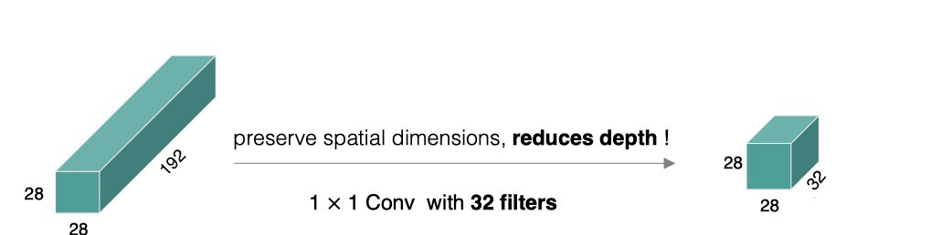
它的作用主要是:
- 跨渠道互动、信息融合
[En]
Cross-channel interaction and information integration*
- 减少和增加卷积核通道数,减少网络参数
[En]
reduce and increase the number of convolution kernel channels and reduce network parameters*
为什么1×1卷积可以减少网络参数?
以inception模块为例,来说明1×1的卷积如何来减少模型参数:
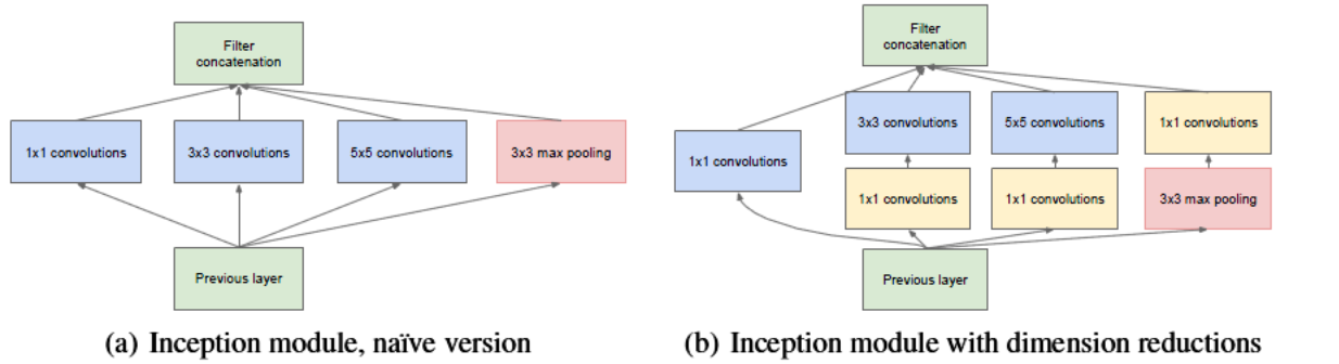
(a)是未加入1×1卷积的inception模块,(b)是加入了1×1 卷积的inception模块。
我们以3×3卷积线路为例,假设输入的特征图大小为(28x28x192),输出特征图的通道数是128:
(a)图中该线路的参数量为:3x3x192x128 = 221184
(b)图中加入1×1卷积后通道为96,再送入3×3卷积中的参数量为:(1x1x192x96)+(3x3x96x128)=129024.
对比可知,加入1×1卷积后参数量减少了。
在tf.keras中实现Inception模块,各个卷积层卷积核的个数通过输入参数来控制,如下所示:
class Inception(tf.keras.layers.Layer):

    def __init__(self, c1, c2, c3, c4):
        super().__init__()

        self.p1_1 = tf.keras.layers.Conv2D(
            c1, kernel_size=1, activation='relu', padding='same')

        self.p2_1 = tf.keras.layers.Conv2D(
            c2[0], kernel_size=1, padding='same', activation='relu')
        self.p2_2 = tf.keras.layers.Conv2D(c2[1], kernel_size=3, padding='same',
                                           activation='relu')

        self.p3_1 = tf.keras.layers.Conv2D(
            c3[0], kernel_size=1, padding='same', activation='relu')
        self.p3_2 = tf.keras.layers.Conv2D(c3[1], kernel_size=5, padding='same',
                                           activation='relu')

        self.p4_1 = tf.keras.layers.MaxPool2D(
            pool_size=3, padding='same', strides=1)
        self.p4_2 = tf.keras.layers.Conv2D(
            c4, kernel_size=1, padding='same', activation='relu')

    def call(self, x):

        p1 = self.p1_1(x)

        p2 = self.p2_2(self.p2_1(x))

        p3 = self.p3_2(self.p3_1(x))

        p4 = self.p4_2(self.p4_1(x))

        outputs = tf.concat([p1, p2, p3, p4], axis=-1)
        return outputs
指定通道数,对Inception模块进行实例化:
Inception(64, (96, 128), (16, 32), 32)
GoogLeNet模型
GoogLeNet主要由Inception模块构成,如下图所示:
整个网络架构分为五个模块,每个模块使用一个3×3的最大池层,跨度为2,以减小输出高度和宽度。
[En]
The whole network architecture is divided into five modules, and each module uses a 3 × 3 maximum pool layer with a stride of 2 to reduce the output height and width.
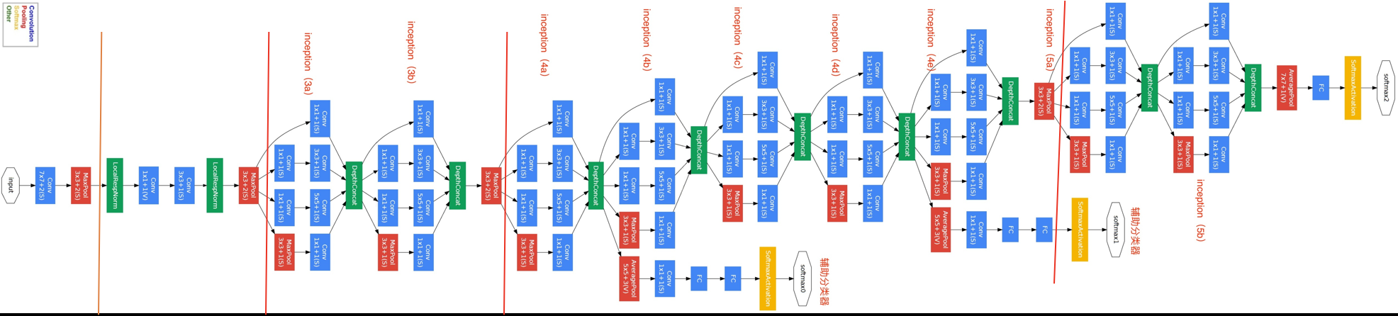
googLeNet的网络设计
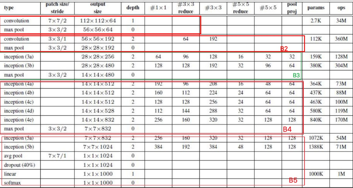
; B1模块
第一模块使用一个64通道的7×7卷积层。
inputs = tf.keras.Input(shape=(224,224,3),name = "input")

x = tf.keras.layers.Conv2D(64, kernel_size=7, strides=2, padding='same', activation='relu')(inputs)

x = tf.keras.layers.MaxPool2D(pool_size=3, strides=2, padding='same')(x)
B2模块
第二模块使用2个卷积层:首先是64通道的1×1卷积层,然后是将通道增大3倍的3×3卷积层。
x = tf.keras.layers.Conv2D(64, kernel_size=1, padding='same', activation='relu')(x)

x = tf.keras.layers.Conv2D(192, kernel_size=3, padding='same', activation='relu')(x)

x = tf.keras.layers.MaxPool2D(pool_size=3, strides=2, padding='same')(x)
B3模块
第三模块串联2个完整的Inception块。第一个Inception块的输出通道数为64+128+32+32=256。第二个Inception块输出通道数增至128+192+96+64=480。
x = Inception(64, (96, 128), (16, 32), 32)(x)

x = Inception(128, (128, 192), (32, 96), 64)(x)

x = tf.keras.layers.MaxPool2D(pool_size=3, strides=2, padding='same')(x)
B4模块
第四模块更加复杂。它串联了5个Inception块,其输出通道数分别是192+208+48+64=512、160+224+64+64=512、128+256+64+64=512、112+288+64+64=528和256+320+128+128=832。并且增加了辅助分类器,根据实验发现网络的中间层具有很强的识别能力,为了利用中间层抽象的特征,在某些中间层中添加含有多层的分类器,如下图所示:
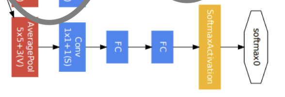
实现如下所示:
def aux_classifier(x, filter_size):

    x = tf.keras.layers.AveragePooling2D(
        pool_size=5, strides=3, padding='same')(x)

    x = tf.keras.layers.Conv2D(filters=filter_size[0], kernel_size=1, strides=1,
                               padding='valid', activation='relu')(x)

    x = tf.keras.layers.Flatten()(x)

    x = tf.keras.layers.Dense(units=filter_size[1], activation='relu')(x)

    x = tf.keras.layers.Dense(units=10, activation='softmax')(x)
    return x
b4模块的实现:
x = Inception(192, (96, 208), (16, 48), 64)(x)

aux_output_1 = aux_classifier(x, [128, 1024])

x = Inception(160, (112, 224), (24, 64), 64)(x)

x = Inception(128, (128, 256), (24, 64), 64)(x)

x = Inception(112, (144, 288), (32, 64), 64)(x)

aux_output_2 = aux_classifier(x, [128, 1024])

x = Inception(256, (160, 320), (32, 128), 128)(x)

x = tf.keras.layers.MaxPool2D(pool_size=3, strides=2, padding='same')(x)
B5模块
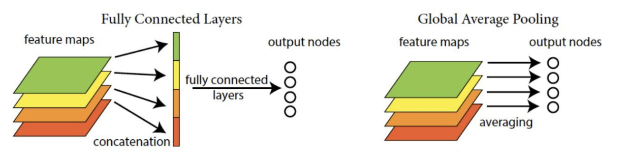
第五模块有输出通道数为256+320+128+128=832和384+384+128+128=1024的两个Inception块。后面紧跟输出层,该模块使用全局平均池化层(GAP)来将每个通道的高和宽变成1。最后输出变成二维数组后接输出个数为标签类别数的全连接层。
全局平均池化层(GAP)
用来替代全连接层前的Flatten,将特征图每一通道中所有像素值相加后求平均,得到就是GAP的结果,在将其送入后续网络中进行计算
实现过程是:
x = Inception(256, (160, 320), (32, 128), 128)(x)

x = Inception(384, (192, 384), (48, 128), 128)(x)

x = tf.keras.layers.GlobalAvgPool2D()(x)

main_outputs = tf.keras.layers.Dense(10,activation='softmax')(x)
构建GoogLeNet模型并通过summary来看下模型的结构:
model = tf.keras.Model(inputs=inputs, outputs=[main_outputs,aux_output_1,aux_output_2])
model.summary()
Model: "functional_3"
_________________________________________________________________
Layer (type)                 Output Shape              Param
=================================================================
input (InputLayer)           [(None, 224, 224, 3)]     0
_________________________________________________________________
conv2d_122 (Conv2D)          (None, 112, 112, 64)      9472
_________________________________________________________________
max_pooling2d_27 (MaxPooling (None, 56, 56, 64)        0
_________________________________________________________________
conv2d_123 (Conv2D)          (None, 56, 56, 64)        4160
_________________________________________________________________
conv2d_124 (Conv2D)          (None, 56, 56, 192)       110784
_________________________________________________________________
max_pooling2d_28 (MaxPooling (None, 28, 28, 192)       0
_________________________________________________________________
inception_19 (Inception)     (None, 28, 28, 256)       163696
_________________________________________________________________
inception_20 (Inception)     (None, 28, 28, 480)       388736
_________________________________________________________________
max_pooling2d_31 (MaxPooling (None, 14, 14, 480)       0
_________________________________________________________________
inception_21 (Inception)     (None, 14, 14, 512)       376176
_________________________________________________________________
inception_22 (Inception)     (None, 14, 14, 512)       449160
_________________________________________________________________
inception_23 (Inception)     (None, 14, 14, 512)       510104
_________________________________________________________________
inception_24 (Inception)     (None, 14, 14, 528)       605376
_________________________________________________________________
inception_25 (Inception)     (None, 14, 14, 832)       868352
_________________________________________________________________
max_pooling2d_37 (MaxPooling (None, 7, 7, 832)         0
_________________________________________________________________
inception_26 (Inception)     (None, 7, 7, 832)         1043456
_________________________________________________________________
inception_27 (Inception)     (None, 7, 7, 1024)        1444080
_________________________________________________________________
global_average_pooling2d_2 ( (None, 1024)              0
_________________________________________________________________
dense_10 (Dense)             (None, 10)                10250
=================================================================
Total params: 5,983,802
Trainable params: 5,983,802
Non-trainable params: 0
___________________________________________________________
手写数字识别
因为ImageNet数据集较大训练时间较长,我们仍用前面的MNIST数据集来演示GoogLeNet。读取数据的时将图像高和宽扩大到图像高和宽224。这个通过 tf.image.resize_with_pad来实现。
数据读取
首先获取数据,并进行维度调整:
import numpy as np

(train_images, train_labels), (test_images, test_labels) = mnist.load_data()

train_images = np.reshape(train_images,(train_images.shape[0],train_images.shape[1],train_images.shape[2],1))

test_images = np.reshape(test_images,(test_images.shape[0],test_images.shape[1],test_images.shape[2],1))
由于使用全部数据训练时间较长,我们定义两个方法获取部分数据,并将图像调整为224*224大小,进行模型训练:(与VGG中是一样的)
def get_train(size):

    index = np.random.randint(0, np.shape(train_images)[0], size)

    resized_images = tf.image.resize_with_pad(train_images[index],224,224,)

    return resized_images.numpy(), train_labels[index]

def get_test(size):

    index = np.random.randint(0, np.shape(test_images)[0], size)

    resized_images = tf.image.resize_with_pad(test_images[index],224,224,)

    return resized_images.numpy(), test_labels[index]
调用上述两种方法,获取参与模型训练和测试的数据集:
[En]
Call the above two methods to get the datasets that participate in model training and testing:
train_images,train_labels = get_train(256)
test_images,test_labels = get_test(128)
模型编译
optimizer = tf.keras.optimizers.SGD(learning_rate=0.01, momentum=0.0)

net.compile(optimizer=optimizer,
              loss='sparse_categorical_crossentropy',
              metrics=['accuracy'],loss_weights=[1,0.3,0.3])
模型训练
net.fit(train_images,train_labels,batch_size=128,epochs=3,verbose=1,validation_split=0.1)
训练过程:
Epoch 1/3
2/2 [==============================] - 8s 4s/step - loss: 2.9527 - accuracy: 0.1174 - val_loss: 3.3254 - val_accuracy: 0.1154
Epoch 2/3
2/2 [==============================] - 7s 4s/step - loss: 2.8111 - accuracy: 0.0957 - val_loss: 2.2718 - val_accuracy: 0.2308
Epoch 3/3
2/2 [==============================] - 7s 4s/step - loss: 2.3055 - accuracy: 0.0957 - val_loss: 2.2669 - val_accuracy: 0.2308
模型评估
net.evaluate(test_images,test_labels,verbose=1)
输出为:
4/4 [==============================] - 1s 338ms/step - loss: 2.3110 - accuracy: 0.0781
[2.310971260070801, 0.078125]
延伸版本
GoogLeNet是以InceptionV1为基础进行构建的,所以GoogLeNet也叫做InceptionNet,在随后的⼏年⾥,研究⼈员对GoogLeNet进⾏了数次改进, 就又产生了InceptionV2,V3,V4等版本。
InceptionV2
在InceptionV2中将大卷积核拆分为小卷积核,将V1中的5×5的卷积用两个3×3的卷积替代,从而增加网络的深度,减少了参数。
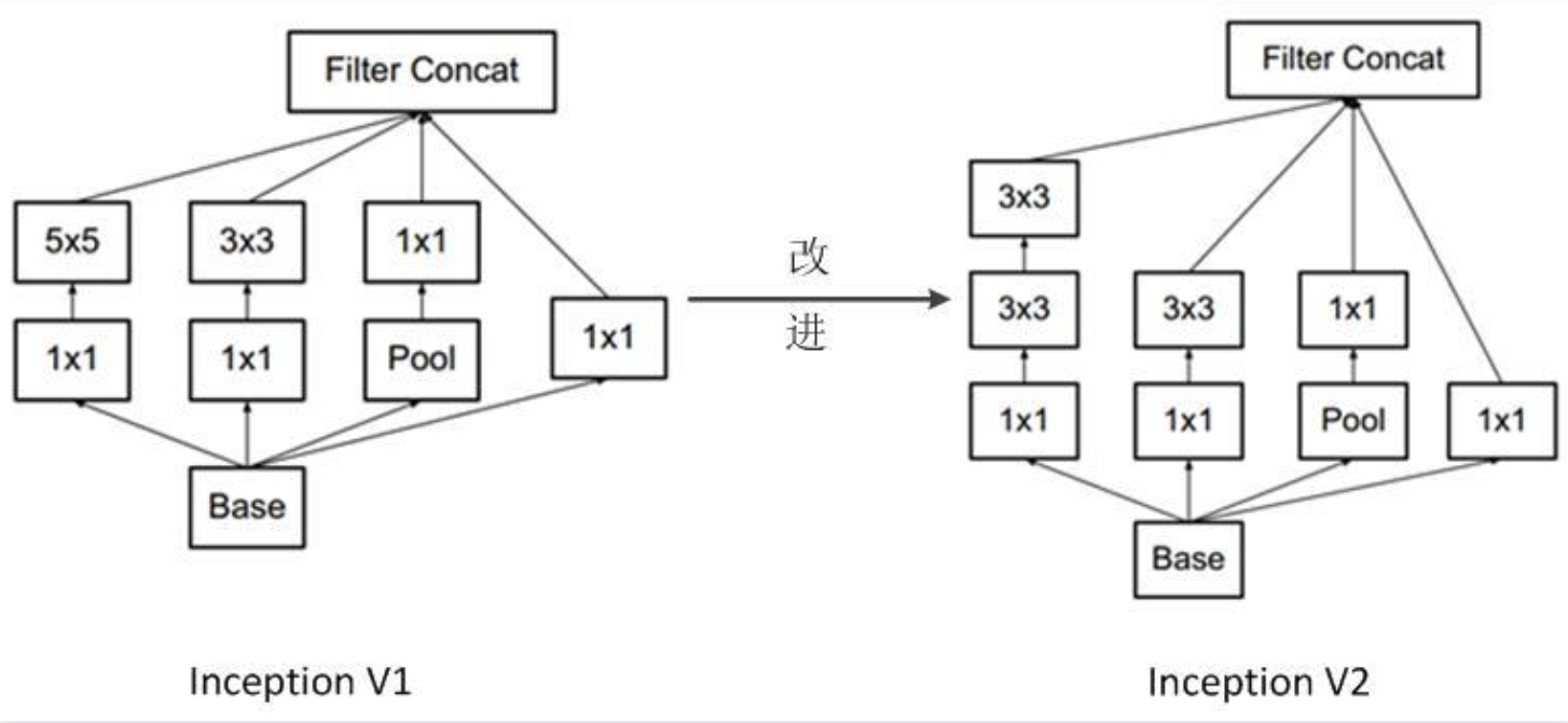
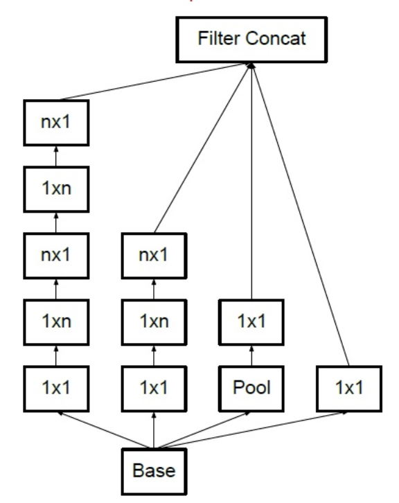
; InceptionV3
将n×n卷积分割为1×n和n×1两个卷积,例如,一个的3×3卷积首先执行一个1×3的卷积,然后执行一个3×1的卷积,这种方法的参数量和计算量都比原来降低。
ResNet
学习目标
- 知道ResNet网络结构的特点
- 能够利用ResNet完成图像分类
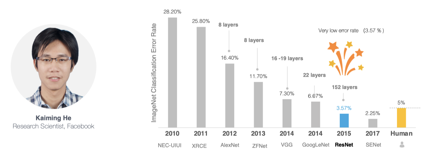
网络越深入,获取的信息和特征就越多。但在实际应用中,随着网络的深入,优化效果变差,测试数据和训练数据的准确性降低。
[En]
The deeper the network, the more information and features are obtained. However, in practice, with the deepening of the network, the optimization effect is worse, and the accuracy of test data and training data is reduced.
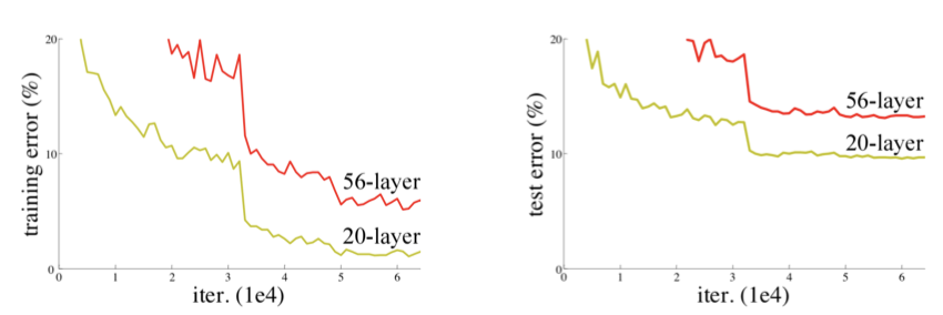
针对这一问题,何恺明等人提出了残差网络(ResNet)在2015年的ImageNet图像识别挑战赛夺魁,并深刻影响了后来的深度神经网络的设计。
; 残差块
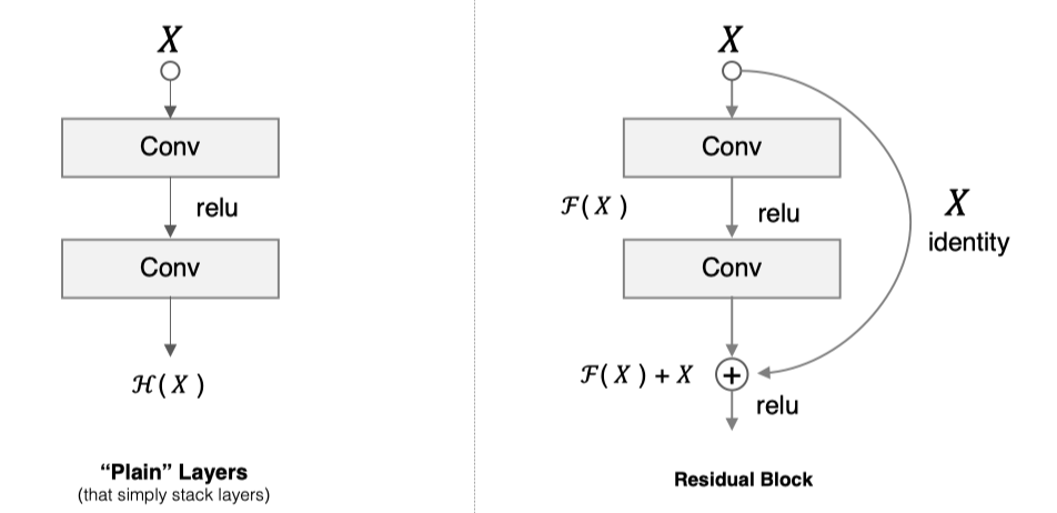
假设 F(x) 代表某个只包含有两层的映射函数, x 是输入, F(x)是输出。假设他们具有相同的维度。在训练的过程中我们希望能够通过修改网络中的 w和b去拟合一个理想的 H(x)(从输入到输出的一个理想的映射函数)。也就是我们的目标是修改F(x) 中的 w和b逼近 H(x) 。如果我们改变思路,用F(x) 来逼近 H(x)-x ,那么我们最终得到的输出就变为 F(x)+x(这里的加指的是对应位置上的元素相加,也就是element-wise addition),这里将直接从输入连接到输出的结构也称为shortcut,那整个结构就是残差块,ResNet的基础模块。
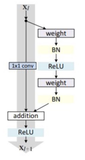
ResNet沿用了VGG全3×33×3卷积层的设计。残差块里首先有2个有相同输出通道数的3×33×3卷积层。每个卷积层后接BN层和ReLU激活函数,然后将输入直接加在最后的ReLU激活函数前,这种结构用于层数较少的神经网络中,比如ResNet34。若输入通道数比较多,就需要引入1×11×1卷积层来调整输入的通道数,这种结构也叫作瓶颈模块,通常用于网络层数较多的结构中。如下图所示:
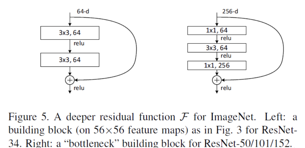
上图左中角残差块的实现如下,可以设置输出通道数、是否使用1:1卷积以及卷积层的步长。
[En]
The implementation of the residual block in the middle left of the image above is as follows, you can set the number of output channels, whether to use 1: 1 convolution and the stride of the convolution layer.
import tensorflow as tf
from tensorflow.keras import layers, activations

class Residual(tf.keras.Model):

    def __init__(self, num_channels, use_1x1conv=False, strides=1):
        super(Residual, self).__init__()

        self.conv1 = layers.Conv2D(num_channels,
                                   padding='same',
                                   kernel_size=3,
                                   strides=strides)

        self.conv2 = layers.Conv2D(num_channels, kernel_size=3, padding='same')
        if use_1x1conv:
            self.conv3 = layers.Conv2D(num_channels,
                                       kernel_size=1,
                                       strides=strides)
        else:
            self.conv3 = None

        self.bn1 = layers.BatchNormalization()
        self.bn2 = layers.BatchNormalization()

    def call(self, X):

        Y = activations.relu(self.bn1(self.conv1(X)))

        Y = self.bn2(self.conv2(Y))

        if self.conv3:
            X = self.conv3(X)

        return activations.relu(Y + X)
1*1卷积用来调整通道数。
ResNet模型
ResNet模型的构成如下图所示:
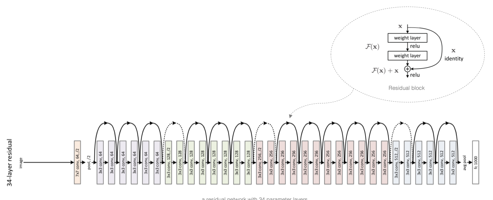
ResNet网络中按照残差块的通道数分为不同的模块。第一个模块前使用了步幅为2的最大池化层,所以无须减小高和宽。之后的每个模块在第一个残差块里将上一个模块的通道数翻倍,并将高和宽减半。
让我们实现这些模块。请注意,这里专门处理了第一个模块。
[En]
Let’s implement these modules. Note that the first module is specially handled here.
class ResnetBlock(tf.keras.layers.Layer):

    def __init__(self,num_channels, num_residuals, first_block=False):
        super(ResnetBlock, self).__init__()

        self.listLayers=[]

        for i in range(num_residuals):

            if i == 0 and not first_block:
                self.listLayers.append(Residual(num_channels, use_1x1conv=True, strides=2))

            else:
                self.listLayers.append(Residual(num_channels))

    def call(self, X):

        for layer in self.listLayers.layers:
            X = layer(X)
        return X
ResNet的前两层跟之前介绍的GoogLeNet中的一样:在输出通道数为64、步幅为2的7×77×7卷积层后接步幅为2的3×33×3的最大池化层。不同之处在于ResNet每个卷积层后增加了BN层,接着是所有残差模块,最后,与GoogLeNet一样,加入全局平均池化层(GAP)后接上全连接层输出。
class ResNet(tf.keras.Model):

    def __init__(self,num_blocks):
        super(ResNet, self).__init__()

        self.conv=layers.Conv2D(64, kernel_size=7, strides=2, padding='same')

        self.bn=layers.BatchNormalization()

        self.relu=layers.Activation('relu')

        self.mp=layers.MaxPool2D(pool_size=3, strides=2, padding='same')

        self.resnet_block1=ResnetBlock(64,num_blocks[0], first_block=True)

        self.resnet_block2=ResnetBlock(128,num_blocks[1])

        self.resnet_block3=ResnetBlock(256,num_blocks[2])

        self.resnet_block4=ResnetBlock(512,num_blocks[3])

        self.gap=layers.GlobalAvgPool2D()

        self.fc=layers.Dense(units=10,activation=tf.keras.activations.softmax)

    def call(self, x):

        x=self.conv(x)

        x=self.bn(x)

        x=self.relu(x)

        x=self.mp(x)

        x=self.resnet_block1(x)
        x=self.resnet_block2(x)
        x=self.resnet_block3(x)
        x=self.resnet_block4(x)

        x=self.gap(x)

        x=self.fc(x)
        return x

mynet=ResNet([2,2,2,2])
这里每个模块里有4个卷积层(不计算 1×1卷积层),加上最开始的卷积层和最后的全连接层,共计18层。这个模型被称为ResNet-18。通过配置不同的通道数和模块里的残差块数可以得到不同的ResNet模型,例如更深的含152层的ResNet-152。虽然ResNet的主体架构跟GoogLeNet的类似,但ResNet结构更简单,修改也更方便。这些因素都导致了ResNet迅速被广泛使用。 在训练ResNet之前,我们来观察一下输入形状在ResNe的架构:
X = tf.random.uniform(shape=(1,  224, 224 , 1))
y = mynet(X)
mynet.summary()
Model: "res_net"
_________________________________________________________________
Layer (type)                 Output Shape              Param
=================================================================
conv2d_2 (Conv2D)            multiple                  3200
_________________________________________________________________
batch_normalization_2 (Batch multiple                  256
_________________________________________________________________
activation (Activation)      multiple                  0
_________________________________________________________________
max_pooling2d (MaxPooling2D) multiple                  0
_________________________________________________________________
resnet_block (ResnetBlock)   multiple                  148736
_________________________________________________________________
resnet_block_1 (ResnetBlock) multiple                  526976
_________________________________________________________________
resnet_block_2 (ResnetBlock) multiple                  2102528
_________________________________________________________________
resnet_block_3 (ResnetBlock) multiple                  8399360
_________________________________________________________________
global_average_pooling2d (Gl multiple                  0
_________________________________________________________________
dense (Dense)                multiple                  5130
=================================================================
Total params: 11,186,186
Trainable params: 11,178,378
Non-trainable params: 7,808
_________________________________________________________________
手写数字势识别
因为ImageNet数据集较大训练时间较长,我们仍用前面的MNIST数据集来演示resNet。读取数据的时将图像高和宽扩大到ResNet使用的图像高和宽224。这个通过 tf.image.resize_with_pad来实现。
数据读取
首先获取数据,并进行维度调整:
import numpy as np

(train_images, train_labels), (test_images, test_labels) = mnist.load_data()

train_images = np.reshape(train_images,(train_images.shape[0],train_images.shape[1],train_images.shape[2],1))

test_images = np.reshape(test_images,(test_images.shape[0],test_images.shape[1],test_images.shape[2],1))
由于使用全部数据进行训练需要较长的时间,因此我们定义了两种方法来获取部分数据,并将图像调整为224到224进行模型训练:
[En]
Because it takes a long time to train with all the data, we define two methods to obtain some of the data, and adjust the image to 224 to 224 for model training:
def get_train(size):

    index = np.random.randint(0, np.shape(train_images)[0], size)

    resized_images = tf.image.resize_with_pad(train_images[index],224,224,)

    return resized_images.numpy(), train_labels[index]

def get_test(size):

    index = np.random.randint(0, np.shape(test_images)[0], size)

    resized_images = tf.image.resize_with_pad(test_images[index],224,224,)

    return resized_images.numpy(), test_labels[index]
调用上述两种方法,获取参与模型训练和测试的数据集:
[En]
Call the above two methods to get the datasets that participate in model training and testing:
train_images,train_labels = get_train(256)
test_images,test_labels = get_test(128)
模型编译
optimizer = tf.keras.optimizers.SGD(learning_rate=0.01, momentum=0.0)

mynet.compile(optimizer=optimizer,
              loss='sparse_categorical_crossentropy',
              metrics=['accuracy'])
模型训练
mynet.fit(train_images,train_labels,batch_size=128,epochs=3,verbose=1,validation_split=0.1)
训练输出为:
Epoch 1/3
2/2 [==============================] - 10s 5s/step - loss: 2.7811 - accuracy: 0.1391 - val_loss: 4.7931 - val_accuracy: 0.1923
Epoch 2/3
2/2 [==============================] - 8s 4s/step - loss: 2.2579 - accuracy: 0.2478 - val_loss: 2.9262 - val_accuracy: 0.2692
Epoch 3/3
2/2 [==============================] - 15s 7s/step - loss: 2.0874 - accuracy: 0.2609 - val_loss: 2.5882 - val_accuracy: 0.2692
模型评估
mynet.evaluate(test_images,test_labels,verbose=1)
输出为:
4/4 [==============================] - 1s 370ms/step - loss: 3.4343 - accuracy: 0.1016
[3.4342570304870605, 0.1015625]
Original: https://blog.csdn.net/qq_43966129/article/details/123075180
Author: 最白の白菜
Title: 经典的图像分类模型
原创文章受到原创版权保护。转载请注明出处:https://www.johngo689.com/497165/
转载文章受原作者版权保护。转载请注明原作者出处!