

array([[0.e+00, 0.e+00, 0.e+00, 0.e+00, 0.e+00, 0.e+00, 0.e+00, 0.e+00],
       [1.e+00, 1.e+00, 1.e-01, 1.e-01, 1.e-02, 1.e-02, 1.e-03, 1.e-03],
       [2.e+00, 2.e+00, 2.e-01, 2.e-01, 2.e-02, 2.e-02, 2.e-03, 2.e-03],
       [3.e+00, 3.e+00, 3.e-01, 3.e-01, 3.e-02, 3.e-02, 3.e-03, 3.e-03]])
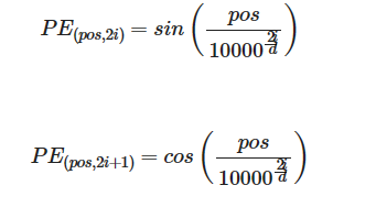
1.2 – 正弦和余弦位置编码
现在,您可以使用计算的角度来计算正弦和余弦位置编码。

练习 2 – 位置编码
实现函数 positional_encoding() 来计算正弦和余弦位置编码
- np.newaxis 有用,具体取决于您选择的实现。就是将矩阵升维
def positional_encoding(positions, d):
"""
    预先计算包含所有位置编码的矩阵

    Arguments:
        positions (int) -- 要编码的最大位置数
        d (int) --编码大小

    Returns:
        pos_encoding -- (1, position, d_model)具有位置编码的矩阵
"""
    # 初始化所有角度angle_rads矩阵
    angle_rads = get_angles(np.arange(positions)[:, np.newaxis],
                            np.arange(d)[ np.newaxis,:],
                            d)

    # -> angle_rads has dim (positions,d)
    # 将 sin 应用于数组中的偶数索引;2i
    angle_rads[:, 0::2] = np.sin(angle_rads[:, 0::2])

    # a将 cos 应用于数组中的偶数索引;2i; 2i+1
    angle_rads[:, 1::2] = np.cos(angle_rads[:, 1::2])
    # END CODE HERE

    pos_encoding = angle_rads[np.newaxis, ...]

    return tf.cast(pos_encoding, dtype=tf.float32)
我们来测试一下:
def positional_encoding_test(target):
    position = 8
    d_model = 16

    pos_encoding = target(position, d_model)
    sin_part = pos_encoding[:, :, 0::2]
    cos_part = pos_encoding[:, :, 1::2]

    assert tf.is_tensor(pos_encoding), "输出不是一个张量"
    assert pos_encoding.shape == (1, position, d_model), f"防止错误,我们希望: (1, {position}, {d_model})"

    ones = sin_part ** 2  +  cos_part ** 2
    assert np.allclose(ones, np.ones((1, position, d_model // 2))), "平方和一定等于1 = sin(a)**2 + cos(a)**2"

    angs = np.arctan(sin_part / cos_part)
    angs[angs < 0] += np.pi
    angs[sin_part.numpy() < 0] += np.pi
    angs = angs % (2 * np.pi)

    pos_m = np.arange(position)[:, np.newaxis]
    dims = np.arange(d_model)[np.newaxis, :]

    trueAngs = get_angles(pos_m, dims, d_model)[:, 0::2] % (2 * np.pi)

    assert np.allclose(angs[0], trueAngs), "您是否分别将 sin 和 cos 应用于偶数和奇数部分?"

    print("\033[92mAll tests passed")

positional_encoding_test(positional_encoding)
All tests passed计算位置编码的工作很好!现在,您可以可视化它们。
pos_encoding = positional_encoding(50, 512)

print (pos_encoding.shape)

plt.pcolormesh(pos_encoding[0], cmap='RdBu')
plt.xlabel('d')
plt.xlim((0, 512))
plt.ylabel('Position')
plt.colorbar()
plt.show()
(1, 50, 512)

每一行代表一个位置编码 – 请注意,没有一行是相同的!您已为每个单词创建了唯一的位置编码。
2 – 掩码
构建transformer网络时,有两种类型的掩码很有用:填充掩码和前瞻掩码。两者都有助于softmax计算为输入句子中的单词提供适当的权重。
2.1 – 填充掩码
通常,输入序列会超过网络可以处理的序列的最大长度。假设模型的最大长度为 5,则按以下序列馈送:
[["Do", "you", "know", "when", "Jane", "is", "going", "to", "visit", "Africa"],
 ["Jane", "visits", "Africa", "in", "September" ],
 ["Exciting", "!"]
]
可能会被矢量化为:
[[ 71, 121, 4, 56, 99, 2344, 345, 1284, 15],
[ 56, 1285, 15, 181, 545],
[ 87, 600]
]<br>将序列传递到转换器模型中时,它们必须具有统一的长度。您可以通过用零填充序列并截断超过模型最大长度的句子来实现此目的:
[[ 71, 121, 4, 56, 99],
[ 2344, 345, 1284, 15, 0],
[ 56, 1285, 15, 181, 545],
[ 87, 600, 0, 0, 0],
]<br>长度超过最大长度 5 的序列将被截断,零将被添加到截断的序列中以实现一致的长度。同样,对于短于最大长度的序列,它们也将添加零以进行填充。<br>但是,这些零会影响softmax计算 - 这是填充掩码派上用场的时候!通过将填充掩码乘以 -1e9 并将其添加到序列中,<br>您可以通过将零设置为接近负无穷大来屏蔽零。我们将为您实现这一点,以便您可以获得构建transformer网络的乐趣!😇 只需确保完成代码,以便在构建模型时正确实现填充。
屏蔽后,您的输入应从 [87, 600, 0, 0, 0] 变为 [87, 600, -1e9, -1e9, -1e9],这样当您采用 softmax 时,零不会影响分数。
def create_padding_mask(seq):
"""
   为填充单元格创建矩阵掩码

    Arguments:
        seq -- (n, m) 矩阵

    Returns:
        mask -- (n, 1, 1, m)二元张量
"""
    #tf.math.equal(a,b) 表示a,b是否相等
    #tf.cast(a,tf.float32) 是将a转化为tf.float32类型
    seq = tf.cast(tf.math.equal(seq, 0), tf.float32)

    # 添加额外尺寸以添加填充
    # to the attention logits.

    return seq[:, tf.newaxis, tf.newaxis, :]
我们测试一下:
x = tf.constant([[7., 6., 0., 0., 1.], [1., 2., 3., 0., 0.], [0., 0., 0., 4., 5.]])
print(create_padding_mask(x))
tf.Tensor(
[[[[0. 0. 1. 1. 0.]]]

 [[[0. 0. 0. 1. 1.]]]

 [[[1. 1. 1. 0. 0.]]]], shape=(3, 1, 1, 5), dtype=float32)如果我们将这个掩码乘以 -1e9 并将其添加到样本输入序列中,则零基本上设置为负无穷大。请注意采用原始序列和掩码序列的softmax时的差异:
print(tf.keras.activations.softmax(x))
print(tf.keras.activations.softmax(x + create_padding_mask(x) * -1.0e9))
tf.Tensor(
[[7.2876632e-01 2.6809818e-01 6.6454883e-04 6.6454883e-04 1.8064311e-03]
 [8.4437370e-02 2.2952460e-01 6.2391245e-01 3.1062772e-02 3.1062772e-02]
 [4.8541022e-03 4.8541022e-03 4.8541022e-03 2.6502502e-01 7.2041267e-01]], shape=(3, 5), dtype=float32)
tf.Tensor(
[[[[7.2973621e-01 2.6845497e-01 0.0000000e+00 0.0000000e+00
    1.8088353e-03]
   [2.4472848e-01 6.6524088e-01 0.0000000e+00 0.0000000e+00
    9.0030566e-02]
   [6.6483547e-03 6.6483547e-03 0.0000000e+00 0.0000000e+00
    9.8670328e-01]]]

 [[[7.3057157e-01 2.6876229e-01 6.6619500e-04 0.0000000e+00
    0.0000000e+00]
   [9.0030566e-02 2.4472848e-01 6.6524088e-01 0.0000000e+00
    0.0000000e+00]
   [3.3333334e-01 3.3333334e-01 3.3333334e-01 0.0000000e+00
    0.0000000e+00]]]

 [[[0.0000000e+00 0.0000000e+00 0.0000000e+00 2.6894143e-01
    7.3105854e-01]
   [0.0000000e+00 0.0000000e+00 0.0000000e+00 5.0000000e-01
    5.0000000e-01]
   [0.0000000e+00 0.0000000e+00 0.0000000e+00 2.6894143e-01
    7.3105854e-01]]]], shape=(3, 1, 3, 5), dtype=float32)
2.2 – 前瞻掩码
前瞻面具遵循类似的直觉。在训练中,您将可以访问训练示例的完整正确输出。前瞻掩码可帮助模型假装它正确预测了部分输出,并查看它是否可以在不向前看的情况下正确预测下一个输出。
例如,如果预期的正确输出是 [1, 2, 3],并且您希望查看给定模型是否正确预测了第一个值,它是否可以预测第二个值,则可以屏蔽第二个和第三个值。因此,您将输入屏蔽序列 [1, -1e9, -1e9],看看它是否可以生成 [1, 2, -1e9]。
仅仅因为你这么努力,我们也会为你😇😇实现这个掩码。同样,请仔细查看代码,以便以后可以有效地实现它。
def create_look_ahead_mask(size):
"""
    返回一个填充有 1 的上三角矩阵

    Arguments:
        size -- 矩阵大小

    Returns:
        mask -- (size, size) 张量
"""
    #tf.linalg.band_part 以对角线为中心,取它的副对角线部分,其他部分用0填充
    mask = tf.linalg.band_part(tf.ones((size, size)), -1, 0)
    return mask
我们来测试一下:
x = tf.random.uniform((1, 3))
temp = create_look_ahead_mask(x.shape[1])
3 – 自注意力
正如变形金刚论文的作者所说,”注意力就是你所需要的一切”。
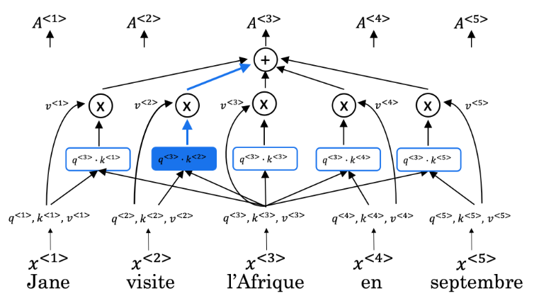
使用与传统卷积网络配对的自我注意允许平行化,从而加快训练速度。您将实现缩放的点积注意力,它将查询、键、值和掩码作为输入,以返回序列中单词的丰富的、基于注意力的矢量表示。这种类型的自我注意可以在数学上表示为:

- Q是查询矩阵
- K是键的矩阵
- V是值的矩阵
- M是您选择应用的可选蒙版
- dk是按键的尺寸,用于缩小所有内容,以便 softmax 不会爆炸
练习 3 – scaled_dot_product_attention
实现函数 ‘scaled_dot_product_attention()’ 来创建基于注意力的表示
def scaled_dot_product_attention(q, k, v, mask):
"""
    计算注意力权重。
      Q、K、V 必须具有匹配的前导尺寸。
      k, v 必须具有匹配的倒数第二个维度,即:seq_len_k = seq_len_v。
      面具根据其类型有不同的形状(填充或向前看)
      但它必须是可广播的添加。

    Arguments:
        q -- query shape == (..., seq_len_q, depth)
        k -- key shape == (..., seq_len_k, depth)
        v -- value shape == (..., seq_len_v, depth_v)
        掩码:形状可广播的浮点张量
              自(..., seq_len_q, seq_len_k). Defaults to None.

    Returns:
        output -- attention_weights
"""
    # START CODE HERE

    # Q*K' 内积
    matmul_qk = tf.matmul(q, k, transpose_b=True)

    #  matmul_qk 的规模
    dk = tf.cast(tf.shape(k)[-1], tf.float32)
    scaled_attention_logits = matmul_qk / tf.math.sqrt(dk)

    # 将掩码添加到缩放张量中。
    if mask is not None:
        scaled_attention_logits += (mask * -1e9)

    # softmax 在最后一个轴 (seq_len_k) 上归一化,以便分数
    # 相加等于1
    attention_weights = tf.nn.softmax(scaled_attention_logits, axis=-1)
    # 注意力权重 * V
    output = tf.matmul(attention_weights, v)   # (..., seq_len_q, depth_v)

    # END CODE HERE

    return output, attention_weights
我们来测试一下:
def scaled_dot_product_attention_test(target):
    q = np.array([[1, 0, 1, 1], [0, 1, 1, 1], [1, 0, 0, 1]]).astype(np.float32)
    k = np.array([[1, 1, 0, 1], [1, 0, 1, 1 ], [0, 1, 1, 0], [0, 0, 0, 1]]).astype(np.float32)
    v = np.array([[0, 0], [1, 0], [1, 0], [1, 1]]).astype(np.float32)

    attention, weights = target(q, k, v, None)
    assert tf.is_tensor(weights), "Weights must be a tensor"
    assert tuple(tf.shape(weights).numpy()) == (q.shape[0], k.shape[1]), f"Wrong shape. We expected ({q.shape[0]}, {k.shape[1]})"
    assert np.allclose(weights, [[0.2589478,  0.42693272, 0.15705977, 0.15705977],
                                   [0.2772748,  0.2772748,  0.2772748,  0.16817567],
                                   [0.33620113, 0.33620113, 0.12368149, 0.2039163 ]])

    assert tf.is_tensor(attention), "Output must be a tensor"
    assert tuple(tf.shape(attention).numpy()) == (q.shape[0], v.shape[1]), f"Wrong shape. We expected ({q.shape[0]}, {v.shape[1]})"
    assert np.allclose(attention, [[0.74105227, 0.15705977],
                                   [0.7227253,  0.16817567],
                                   [0.6637989,  0.2039163 ]])

    mask = np.array([[0, 0, 1, 0], [0, 0, 1, 0], [0, 0, 1, 0]])
    attention, weights = target(q, k, v, mask)

    assert np.allclose(weights, [[0.30719590187072754, 0.5064803957939148, 0.0, 0.18632373213768005],
                                 [0.3836517333984375, 0.3836517333984375, 0.0, 0.2326965481042862],
                                 [0.3836517333984375, 0.3836517333984375, 0.0, 0.2326965481042862]]), "Wrong masked weights"
    assert np.allclose(attention, [[0.6928040981292725, 0.18632373213768005],
                                   [0.6163482666015625, 0.2326965481042862],
                                   [0.6163482666015625, 0.2326965481042862]]), "Wrong masked attention"

    print("\033[92mAll tests passed")

scaled_dot_product_attention_test(scaled_dot_product_attention)
出色的工作!您现在可以实现自我关注。有了它,您就可以开始构建编码器块了!
4 – 编码快
转换器编码器层将自我注意和卷积神经网络风格的处理配对,以提高训练速度,并将 K 和 V 矩阵传递给解码器,稍后将在作业中构建解码器。在作业的这一部分中,您将通过配对多头注意力和前馈神经网络来实现编码器(图 2a)。
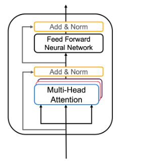
- 多头注意力可以认为是多次计算自我注意力以检测不同的特征。
- 前馈神经网络包含两个密集层,我们将实现为函数全连接
您的输入句子首先通过多头注意力层,编码器在对特定单词进行编码时会查看输入句子中的其他单词。然后将多头注意力层的输出馈送到前馈神经网络。完全相同的前馈网络独立应用于每个位置。
- 对于MultiHeadAttention层,您将使用Keras实现。如果您对如何将查询矩阵 Q、键矩阵 K 和值矩阵 V 拆分为不同的头感到好奇,可以查看实现。
- 您还将使用具有两个密集层的顺序 API 来构建前馈神经网络层。
def FullyConnected(embedding_dim, fully_connected_dim):
    return tf.keras.Sequential([
        tf.keras.layers.Dense(fully_connected_dim, activation='relu'),  # (batch_size, seq_len, dff)
        tf.keras.layers.Dense(embedding_dim)  # (batch_size, seq_len, d_model)
    ])
4.1-编码层
现在,您可以在编码器层中将多头注意力和前馈神经网络配对在一起!您还将使用残差连接和层归一化来帮助加快训练速度(图 2a)。
练习4 – EncoderLayer
使用 call() 方法实现 EncoderLayer()
在本练习中,您将使用 call() 方法实现一个编码器块(图 2)。该函数应执行以下步骤:
- 您将 Q、V、K 矩阵和布尔掩码传递给多头注意力层。请记住,要计算自注意Q,V和K应该是相同的。
- 接下来,您将多头注意力层的输出传递给辍学层。不要忘记使用训练参数来设置模型的模式。
- 现在,通过添加原始输入 x 和 dropout 图层的输出来添加跳过连接。
- 添加跳过连接后,通过第一层规范化传递输出。
- 最后,重复步骤 1-4,但使用前馈神经网络而不是多头注意力层。
其他提示:
- init 方法创建将由调用方法访问的所有层。无论想在哪里使用在 init 方法中定义的层,都必须使用语法 self。[插入图层名称]。
- 您会发现MultiHeadAttention的文档很有帮助。请注意,如果查询、键和值相同,则此函数执行自我注意。
class EncoderLayer(tf.keras.layers.Layer):
"""
    编码器层由多头自注意力机构组成,
    然后是一个简单的、按位置的全连接前馈网络。
    这个拱门包括围绕两者的残余连接
    子层,然后是层归一化。
"""
    def __init__(self, embedding_dim, num_heads, fully_connected_dim, dropout_rate=0.1, layernorm_eps=1e-6):
        super(EncoderLayer, self).__init__()

        self.mha = MultiHeadAttention(num_heads=num_heads,
                                      key_dim=embedding_dim)

        self.ffn = FullyConnected(embedding_dim=embedding_dim,
                                  fully_connected_dim=fully_connected_dim)

        self.layernorm1 = LayerNormalization(epsilon=layernorm_eps)
        self.layernorm2 = LayerNormalization(epsilon=layernorm_eps)

        self.dropout1 = Dropout(dropout_rate)
        self.dropout2 = Dropout(dropout_rate)

    def call(self, x, training, mask):
"""
        编码器层的正向传递

        Arguments:
           x -- 形状张量(batch_size、input_seq_len、embedding_dim)
            训练 -- 布尔值,设置为 true 以激活
                        失活层的训练模式
            掩码 -- 布尔掩码,以确保填充不是
                    被视为输入的一部分
        Returns:
            out2 -- 形状张量(batch_size、input_seq_len、embedding_dim)
"""
        # START CODE HERE
        # 计算自注意力使用 mha(~1 line)
        #-> 要计算自我注意Q,V和K应该相同(x)
        self_attn_output = self.mha(x, x, x, mask) # Self attention (batch_size, input_seq_len, embedding_dim)

        # 将失活层应用于自我注意输出(~1 line)
        self_attn_output = self.dropout1(self_attn_output, training=training)

        # 对输入和注意力输出的总和应用层归一化,以获得
        # 多头注意力层输出 (~1 line)
        mult_attn_out = self.layernorm1(x + self_attn_output)  # (batch_size, input_seq_len, embedding_dim)

        # 通过FFN传递多头注意力层的输出(~1 line)
        ffn_output = self.ffn(mult_attn_out)  # (batch_size, input_seq_len, embedding_dim)

        # 将失活层应用于 FFN 输出 (~1 line)
        ffn_output = self.dropout2(ffn_output, training=training)

        # 对多头注意力和 FFN 输出的输出之和应用层归一化,以获得
        # 编码器层输出(~1 行)
        encoder_layer_out = self.layernorm2(ffn_output + mult_attn_out)  # (batch_size, input_seq_len, embedding_dim)
        # END CODE HERE

        return encoder_layer_out
测试一下吧:
def EncoderLayer_test(target):
    q = np.array([[[1, 0, 1, 1], [0, 1, 1, 1], [1, 0, 0, 1]]]).astype(np.float32)
    encoder_layer1 = EncoderLayer(4, 2, 8)
    tf.random.set_seed(10)
    encoded = encoder_layer1(q, True, np.array([[1, 0, 1]]))

    assert tf.is_tensor(encoded), "Wrong type. Output must be a tensor"
    assert tuple(tf.shape(encoded).numpy()) == (1, q.shape[1], q.shape[2]), f"Wrong shape. We expected ((1, {q.shape[1]}, {q.shape[2]}))"

    assert np.allclose(encoded.numpy(),
                       [[-0.5214877 , -1.001476  , -0.12321664,  1.6461804 ],
                       [-1.3114998 ,  1.2167752 , -0.5830886 ,  0.6778133 ],
                       [ 0.25485858,  0.3776546 , -1.6564771 ,  1.023964  ]],), "Wrong values"

    print("\033[92mAll tests passed")

EncoderLayer_test(EncoderLayer)
All tests passed
4.2 – 全编码器
干得真棒!您现在已经成功实现了位置编码、自我注意和编码器层 – 拍拍自己的背。现在,您已准备好构建完整的变压器编码器(图 2b),您将在其中嵌入输入并添加计算的位置编码。然后,您将编码的嵌入馈送到编码器层堆栈。
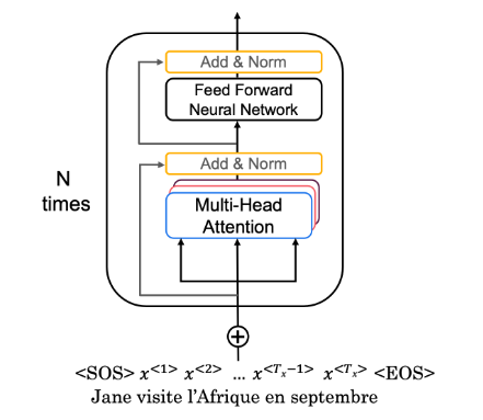
练习 5 – Encoder
使用 call() 方法完成 Encoder() 函数,以嵌入输入、添加位置编码并实现多个编码器层
在本练习中,您将使用嵌入层、位置编码和多个编码器层初始化编码器。您的 call() 方法将执行以下步骤:
- 通过嵌入层传递输入。
- 通过将嵌入乘以嵌入维度的平方根来缩放嵌入。请记住在计算平方根之前将嵌入维度转换为数据类型 tf.float32。
- 将位置编码:self.pos_encoding [:, :seq_len, :] 添加到嵌入中。
- 将编码嵌入传递到一个 dropout 层,记住使用训练参数来设置模型训练模式。
- 使用 for 循环将 dropout 层的输出传递到编码层堆栈。
class Encoder(tf.keras.layers.Layer):
"""
    整个编码器首先将输入传递到嵌入层
    并使用位置编码将输出传递到堆栈
    编码器层

"""
    def __init__(self, num_layers, embedding_dim, num_heads, fully_connected_dim, input_vocab_size,
               maximum_position_encoding, dropout_rate=0.1, layernorm_eps=1e-6):
        super(Encoder, self).__init__()

        self.embedding_dim = embedding_dim
        self.num_layers = num_layers

        self.embedding = Embedding(input_vocab_size, self.embedding_dim)
        self.pos_encoding = positional_encoding(maximum_position_encoding,
                                                self.embedding_dim)

        self.enc_layers = [EncoderLayer(embedding_dim=self.embedding_dim,
                                        num_heads=num_heads,
                                        fully_connected_dim=fully_connected_dim,
                                        dropout_rate=dropout_rate,
                                        layernorm_eps=layernorm_eps)
                           for _ in range(self.num_layers)]

        self.dropout = Dropout(dropout_rate)

    def call(self, x, training, mask):
"""
       编码器的正向传递

        Arguments:
           x -- 形状张量 (batch_size, input_seq_len)
            训练 -- 布尔值,设置为 true 以激活
                        辍学层的训练模式
            掩码 -- 布尔掩码,以确保填充不是
                    被视为输入的一部分
        Returns:
            out2 -- 形状张量(batch_size、input_seq_len、embedding_dim)
"""

        seq_len = tf.shape(x)[1]

        # START CODE HERE
        # 通过嵌入层传递输入
        x = self.embedding(x)  # (batch_size, input_seq_len, embedding_dim)
        # 通过将嵌入乘以嵌入维度的平方根来缩放嵌入
        x *= tf.math.sqrt(tf.cast(self.embedding_dim,tf.float32))
        # 将位置编码添加到嵌入
        x += self.pos_encoding[:, :seq_len, :]
        # 通过失活层传递编码嵌入
        x = self.dropout(x, training=training)
        # 通过编码层堆栈传递输出
        for i in range(self.num_layers):
            x = self.enc_layers[i](x,training, mask)
        # END CODE HERE

        return x  # (batch_size, input_seq_len, embedding_dim)
测试一下吧:
def Encoder_test(target):
    tf.random.set_seed(10)

    embedding_dim=4

    encoderq = target(num_layers=2,
                      embedding_dim=embedding_dim,
                      num_heads=2,
                      fully_connected_dim=8,
                      input_vocab_size=32,
                      maximum_position_encoding=5)

    x = np.array([[2, 1, 3], [1, 2, 0]])

    encoderq_output = encoderq(x, True, None)

    assert tf.is_tensor(encoderq_output), "Wrong type. Output must be a tensor"
    assert tuple(tf.shape(encoderq_output).numpy()) == (x.shape[0], x.shape[1], embedding_dim), f"Wrong shape. We expected ({eshape[0]}, {eshape[1]}, {embedding_dim})"
    assert np.allclose(encoderq_output.numpy(),
                       [[[-0.40172306,  0.11519244, -1.2322885,   1.5188192 ],
                         [ 0.4017268,   0.33922842, -1.6836855,   0.9427304 ],
                         [ 0.4685002,  -1.6252842,   0.09368491,  1.063099  ]],
                        [[-0.3489219,   0.31335592, -1.3568854,   1.3924513 ],
                         [-0.08761203, -0.1680029,  -1.2742313,   1.5298463 ],
                         [ 0.2627198,  -1.6140151,   0.2212624 ,  1.130033  ]]]), "Wrong values"

    print("\033[92mAll tests passed")

Encoder_test(Encoder)
All tests passed
5 – 译码器
解码器层采用编码器生成的 K 和 V 矩阵,并使用输出中的 Q 矩阵计算第二个多头注意力层(图 3a)。
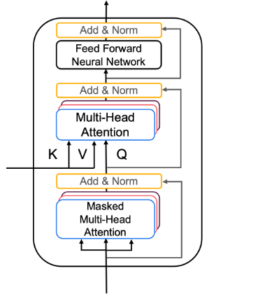
5.1 – 译码器层
同样,您将多头注意力与前馈神经网络配对,但这次您将实现两个多头注意力层。您还将使用残差连接和层归一化来帮助加快训练速度(图 3a)。
练习 6 – DecoderLayer
使用 call() 方法实现解码器层()
- 块 1 是一个多头注意力层,具有残差连接、辍学层和前瞻掩码。
- 模块 2 将考虑编码器的输出,因此多头注意层将从编码器接收 K 和 V,从模块 1 接收 Q。然后,您将应用辍学层、层归一化和残差连接,就像您之前所做的那样。
- 最后,Block 3 是一个具有 dropout 和归一化层以及残差连接的前馈神经网络。
- 前两个块与 EncoderLayer 非常相似,只是在计算自我注意时会返回attention_scores
class DecoderLayer(tf.keras.layers.Layer):
"""
   解码器层由两个多头注意力块组成,
    一个接受新的输入并使用自我注意,另一个
    一个将其与编码器的输出相结合,然后是
    完全连接的块。
"""
    def __init__(self, embedding_dim, num_heads, fully_connected_dim, dropout_rate=0.1, layernorm_eps=1e-6):
        super(DecoderLayer, self).__init__()

        self.mha1 = MultiHeadAttention(num_heads=num_heads,
                                      key_dim=embedding_dim)

        self.mha2 = MultiHeadAttention(num_heads=num_heads,
                                      key_dim=embedding_dim)

        self.ffn = FullyConnected(embedding_dim=embedding_dim,
                                  fully_connected_dim=fully_connected_dim)

        self.layernorm1 = LayerNormalization(epsilon=layernorm_eps)
        self.layernorm2 = LayerNormalization(epsilon=layernorm_eps)
        self.layernorm3 = LayerNormalization(epsilon=layernorm_eps)

        self.dropout1 = Dropout(dropout_rate)
        self.dropout2 = Dropout(dropout_rate)
        self.dropout3 = Dropout(dropout_rate)

    def call(self, x, enc_output, training, look_ahead_mask, padding_mask):
"""
        解码器层的正向传递

        参数:
            x -- 形状张量(batch_size、target_seq_len、embedding_dim)
            enc_output -- 形状张量(batch_size、input_seq_len、embedding_dim)
            训练 -- 布尔值,设置为 true 以激活
                        辍学层的训练模式
            look_ahead_mask -- target_input的布尔掩码
            padding_mask -- 第二个多头注意力层的布尔掩码
        返回:
            out3 -- 形状张量 (batch_size, target_seq_len, embedding_dim)
            attn_weights_block1 -- 形状张量(batch_size、num_heads、target_seq_len、input_seq_len)
            attn_weights_block2 -- 形状张量(batch_size、num_heads、target_seq_len、input_seq_len)
"""

        # START CODE HERE
        # enc_output.shape == (batch_size, input_seq_len, embedding_dim)

        # BLOCK 1
        # 计算自我注意和返回注意力分数为 attn_weights_block1 (~1 行)
        attn1, attn_weights_block1 = self.mha1(x, x, x,look_ahead_mask, return_attention_scores=True)  # (batch_size, target_seq_len, d_model)

        # 在注意力输出上应用失活层(~1 行)
        attn1 = self.dropout1(attn1, training = training)

        # 对注意力输出和输入的总和应用层归一化(~1 行)
        out1 = self.layernorm1(attn1 + x)

        # BLOCK 2
        # 使用来自第一个块的 Q 和来自编码器输出的 K 和 V 计算自我注意。
        # 多头注意力的调用接受输入(查询、值、键、attention_mask、return_attention_scores、训练)
        # 将注意力分数作为attn_weights_block2返回(~1 行)
        attn2, attn_weights_block2 = self.mha2( out1,enc_output, enc_output, padding_mask, return_attention_scores=True)  # (batch_size, target_seq_len, d_model)

        # 在注意力输出上应用失活层(~1 行)
        attn2 = self.dropout2(attn2, training=training)

        # 对注意力输出和第一个块的输出之和应用层归一化(~1 行)
        out2 = self.layernorm2(attn2 + out1)  # (batch_size, target_seq_len, embedding_dim)

        #BLOCK 3
        # 通过 FFN 传递第二个块的输出
        ffn_output = self.ffn(out2) # (batch_size, target_seq_len, embedding_dim)

        # 将辍学图层应用于 FFN 输出
        ffn_output = self.dropout3(ffn_output, training=training)

        # 将层归一化应用于 FFN 输出和第二个块的输出之和
        out3 =  self.layernorm3(ffn_output + out2) # (batch_size, target_seq_len, embedding_dim)
        # END CODE HERE

        return out3, attn_weights_block1, attn_weights_block2
测试一下:
def DecoderLayer_test(target):

    num_heads=8
    tf.random.set_seed(10)

    decoderLayerq = target(
        embedding_dim=4,
        num_heads=num_heads,
        fully_connected_dim=32,
        dropout_rate=0.1,
        layernorm_eps=1e-6)

    encoderq_output = tf.constant([[[-0.40172306,  0.11519244, -1.2322885,   1.5188192 ],
                                   [ 0.4017268,   0.33922842, -1.6836855,   0.9427304 ],
                                   [ 0.4685002,  -1.6252842,   0.09368491,  1.063099  ]]])

    q = np.array([[[1, 0, 1, 1], [0, 1, 1, 1], [1, 0, 0, 1]]]).astype(np.float32)

    look_ahead_mask = tf.constant([[1., 0., 0.],
                       [1., 1., 0.],
                       [1., 1., 1.]])

    padding_mask = None
    out, attn_w_b1, attn_w_b2 = decoderLayerq(q, encoderq_output, True, look_ahead_mask, padding_mask)

    assert tf.is_tensor(attn_w_b1), "Wrong type for attn_w_b1. Output must be a tensor"
    assert tf.is_tensor(attn_w_b2), "Wrong type for attn_w_b2. Output must be a tensor"
    assert tf.is_tensor(out), "Wrong type for out. Output must be a tensor"

    shape1 = (q.shape[0], num_heads, q.shape[1], q.shape[1])
    assert tuple(tf.shape(attn_w_b1).numpy()) == shape1, f"Wrong shape. We expected {shape1}"
    assert tuple(tf.shape(attn_w_b2).numpy()) == shape1, f"Wrong shape. We expected {shape1}"
    assert tuple(tf.shape(out).numpy()) == q.shape, f"Wrong shape. We expected {q.shape}"

    assert np.allclose(attn_w_b1[0, 0, 1], [0.5271505,  0.47284946, 0.], atol=1e-2), "Wrong values in attn_w_b1. Check the call to self.mha1"
    assert np.allclose(attn_w_b2[0, 0, 1], [0.33365652, 0.32598493, 0.34035856]),  "Wrong values in attn_w_b2. Check the call to self.mha2"
    assert np.allclose(out[0, 0], [0.04726627, -1.6235218, 1.0327158, 0.54353976]), "Wrong values in out"

    # Now let's try a example with padding mask
    padding_mask = np.array([[0, 0, 1]])
    out, attn_w_b1, attn_w_b2 = decoderLayerq(q, encoderq_output, True, look_ahead_mask, padding_mask)

    assert np.allclose(out[0, 0], [-0.34323323, -1.4689083, 1.1092525, 0.7028891]), "Wrong values in out when we mask the last word. Are you passing the padding_mask to the inner functions?"

    print("\033[92mAll tests passed")

DecoderLayer_test(DecoderLayer)
All tests passed
5.2 – 全译码器
你快到了!是时候使用解码器层构建完整的转换器解码器了(图 3b)。您将嵌入输出并添加位置编码。然后,您将编码的嵌入馈送到解码器层堆栈。
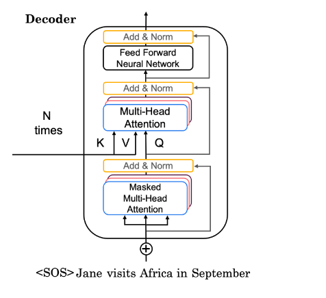
练习7 – Decoder
mplement Decoder() 使用 call() 方法嵌入输出、添加位置编码和实现多个解码器层
在本练习中,您将使用嵌入层、位置编码和多个解码器层初始化解码器。您的 call() 方法将执行以下步骤:
- 通过嵌入层传递生成的输出。
- 通过将嵌入乘以嵌入维度的平方根来缩放嵌入。请记住在计算平方根之前将嵌入维度转换为数据类型 tf.float32。
- 将位置编码:self.pos_encoding [:, :seq_len, :] 添加到嵌入中。
- 将编码嵌入传递到一个 dropout 层,记住使用训练参数来设置模型训练模式。
- 使用 for 循环通过解码层堆栈传递 dropout 层的输出。
class Decoder(tf.keras.layers.Layer):
"""
   整个编码器首先将目标输入传递到嵌入层
    并使用位置编码将输出传递到堆栈
    解码器层

"""
    def __init__(self, num_layers, embedding_dim, num_heads, fully_connected_dim, target_vocab_size,
               maximum_position_encoding, dropout_rate=0.1, layernorm_eps=1e-6):
        super(Decoder, self).__init__()

        self.embedding_dim = embedding_dim
        self.num_layers = num_layers

        self.embedding = Embedding(target_vocab_size, self.embedding_dim)
        self.pos_encoding = positional_encoding(maximum_position_encoding, self.embedding_dim)

        self.dec_layers = [DecoderLayer(embedding_dim=self.embedding_dim,
                                        num_heads=num_heads,
                                        fully_connected_dim=fully_connected_dim,
                                        dropout_rate=dropout_rate,
                                        layernorm_eps=layernorm_eps)
                           for _ in range(self.num_layers)]
        self.dropout = Dropout(dropout_rate)

    def call(self, x, enc_output, training,
           look_ahead_mask, padding_mask):
"""
       解码器的正向传递

参数:
            x -- 形状张量(batch_size、target_seq_len、embedding_dim)
            enc_output -- 形状张量(batch_size、input_seq_len、embedding_dim)
            训练 -- 布尔值,设置为 true 以激活
                        辍学层的训练模式
            look_ahead_mask -- target_input的布尔掩码
            padding_mask -- 第二个多头注意力层的布尔掩码
        返回:
            x -- 形状张量(batch_size、target_seq_len、embedding_dim)
            attention_weights - 包含所有注意力权重的张量字典
                                每个形状 形状的张量(batch_size、num_heads、target_seq_len、input_seq_len)
"""

        seq_len = tf.shape(x)[1]
        attention_weights = {}

        # START CODE HERE
        # 创建单词嵌入
        x = self.embedding(x)  # (batch_size, target_seq_len, embedding_dim)

        # 通过乘以维度的平方根来缩放嵌入
        x *= tf.math.sqrt(tf.cast(self.embedding_dim, tf.float32))

        # 计算位置编码并添加到单词嵌入
        x += self.pos_encoding[:, :seq_len, :]

        # 将失活图层应用于 X
        x = self.dropout(x, training=training)

        # 使用 for 循环通过解码器层堆栈传递 x 并更新attention_weights(总共 ~4 行)
        for i in range(self.num_layers):
            # pASS X和编码器通过一堆解码器层输出,节省注意力权重
            #块 1 和块 2 的 # (~1 行)
            x, block1, block2 = self.dec_layers[i](x, enc_output, training, look_ahead_mask, padding_mask)

            #update attention_weights 字典,具有块 1 和块 2 的注意权重
            attention_weights['decoder_layer{}_block1_self_att'.format(i+1)] = block1
            attention_weights['decoder_layer{}_block2_decenc_att'.format(i+1)] = block2
        # END CODE HERE

        # x.shape == (batch_size, target_seq_len, embedding_dim)
        return x, attention_weights
测试一下:
def Decoder_test(target):

    tf.random.set_seed(10)

    num_layers=7
    embedding_dim=4
    num_heads=3
    fully_connected_dim=8
    target_vocab_size=33
    maximum_position_encoding=6

    x = np.array([[3, 2, 1], [2, 1, 0]])

    encoderq_output = tf.constant([[[-0.40172306,  0.11519244, -1.2322885,   1.5188192 ],
                         [ 0.4017268,   0.33922842, -1.6836855,   0.9427304 ],
                         [ 0.4685002,  -1.6252842,   0.09368491,  1.063099  ]],
                        [[-0.3489219,   0.31335592, -1.3568854,   1.3924513 ],
                         [-0.08761203, -0.1680029,  -1.2742313,   1.5298463 ],
                         [ 0.2627198,  -1.6140151,   0.2212624 ,  1.130033  ]]])

    look_ahead_mask = tf.constant([[1., 0., 0.],
                       [1., 1., 0.],
                       [1., 1., 1.]])

    decoderk = Decoder(num_layers,
                    embedding_dim,
                    num_heads,
                    fully_connected_dim,
                    target_vocab_size,
                    maximum_position_encoding)
    outd, att_weights = decoderk(x, encoderq_output, False, look_ahead_mask, None)

    assert tf.is_tensor(outd), "Wrong type for outd. It must be a dict"
    assert np.allclose(tf.shape(outd), tf.shape(encoderq_output)), f"Wrong shape. We expected { tf.shape(encoderq_output)}"
    print(outd[1, 1])
    assert np.allclose(outd[1, 1], [-0.2715261, -0.5606001, -0.861783, 1.69390933]), "Wrong values in outd"

    keys = list(att_weights.keys())
    assert type(att_weights) == dict, "Wrong type for att_weights[0]. Output must be a tensor"
    assert len(keys) == 2 * num_layers, f"Wrong length for attention weights. It must be 2 x num_layers = {2*num_layers}"
    assert tf.is_tensor(att_weights[keys[0]]), f"Wrong type for att_weights[{keys[0]}]. Output must be a tensor"
    shape1 = (x.shape[0], num_heads, x.shape[1], x.shape[1])
    assert tuple(tf.shape(att_weights[keys[1]]).numpy()) == shape1, f"Wrong shape. We expected {shape1}"
    assert np.allclose(att_weights[keys[0]][0, 0, 1], [0.52145624, 0.47854376, 0.]), f"Wrong values in att_weights[{keys[0]}]"

    print("\033[92mAll tests passed")

Decoder_test(Decoder)
tf.Tensor([-0.2715261 -0.5606004 -0.8617829  1.6939092], shape=(4,), dtype=float32)
All tests passed
6 – Transformer
唷!这是相当艰巨的任务,现在你已经完成了深度学习专业化的最后一次练习。祝贺!你已经完成了所有艰苦的工作,现在是时候把它们放在一起了。
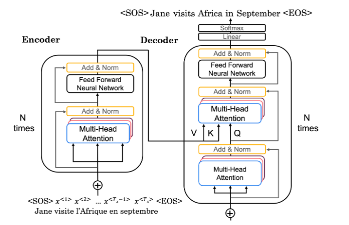
通过转换器体系结构的数据流如下所示:
-
首先,输入通过编码器,该编码器只是您实现的重复编码器层:
-
输入的嵌入和位置编码
- 多头关注您的输入
-
前馈神经网络以帮助检测特征
-
然后,预测的输出通过解码器,解码器由你实现的解码器层组成:
-
输出的嵌入和位置编码
- 对生成的输出进行多头关注
- 多头注意力,Q来自第一个多头注意力层,K和V来自编码器
-
前馈神经网络,帮助检测特征
-
最后,在第 N 个解码器层之后,应用两个密集层和一个 softmax 来生成序列中下一个输出的预测。
练习8 – Transformer
使用 call() 方法实现 Transformer()
- 使用适当的掩码将输入传递到编码器。
- 使用适当的掩码通过解码器传递编码器输出和目标。
- 应用线性变换和软最大值来获得预测。
class Transformer(tf.keras.Model):
"""
    带编码器和解码器的完整transformer
"""
    def __init__(self, num_layers, embedding_dim, num_heads, fully_connected_dim, input_vocab_size,
               target_vocab_size, max_positional_encoding_input,
               max_positional_encoding_target, dropout_rate=0.1, layernorm_eps=1e-6):
        super(Transformer, self).__init__()

        self.encoder = Encoder(num_layers=num_layers,
                               embedding_dim=embedding_dim,
                               num_heads=num_heads,
                               fully_connected_dim=fully_connected_dim,
                               input_vocab_size=input_vocab_size,
                               maximum_position_encoding=max_positional_encoding_input,
                               dropout_rate=dropout_rate,
                               layernorm_eps=layernorm_eps)

        self.decoder = Decoder(num_layers=num_layers,
                               embedding_dim=embedding_dim,
                               num_heads=num_heads,
                               fully_connected_dim=fully_connected_dim,
                               target_vocab_size=target_vocab_size,
                               maximum_position_encoding=max_positional_encoding_target,
                               dropout_rate=dropout_rate,
                               layernorm_eps=layernorm_eps)

        self.final_layer = Dense(target_vocab_size, activation='softmax')

    def call(self, inp, tar, training, enc_padding_mask, look_ahead_mask, dec_padding_mask):
"""
        整个变压器的正向传递
        参数:
            inp -- 形状张量(batch_size、input_seq_len、fully_connected_dim)
            tar -- 形状张量(batch_size、target_seq_len、fully_connected_dim)
            训练 -- 布尔值,设置为 true 以激活
                        辍学层的训练模式
            enc_padding_mask -- 布尔掩码,以确保填充不是
                    被视为输入的一部分
            look_ahead_mask -- target_input的布尔掩码
            padding_mask -- 第二个多头注意力层的布尔掩码
        返回:
            final_output -- 描述我
            attention_weights - 包含解码器所有注意力权重的张量字典
                                每个形状 形状的张量(batch_size、num_heads、target_seq_len、input_seq_len)

"""
        # START CODE HERE
        # 使用适当的参数调用 self.encoder 以获取编码器输出
        enc_output = self.encoder(inp,training,enc_padding_mask) # (batch_size, inp_seq_len, fully_connected_dim)

        # 使用适当的参数调用 self.decoder 以获取解码器输出
        # dec_output.shape == (batch_size, tar_seq_len, fully_connected_dim)
        dec_output, attention_weights = self.decoder(tar, enc_output, training, look_ahead_mask, dec_padding_mask)

        # 通过线性层和softmax(~2行)传递解码器输出
        final_output = self.final_layer(dec_output)  # (batch_size, tar_seq_len, target_vocab_size)
        # START CODE HERE

        return final_output, attention_weights
我们测试一下:
def Transformer_test(target):

    tf.random.set_seed(10)

    num_layers = 6
    embedding_dim = 4
    num_heads = 4
    fully_connected_dim = 8
    input_vocab_size = 30
    target_vocab_size = 35
    max_positional_encoding_input = 5
    max_positional_encoding_target = 6

    trans = Transformer(num_layers,
                        embedding_dim,
                        num_heads,
                        fully_connected_dim,
                        input_vocab_size,
                        target_vocab_size,
                        max_positional_encoding_input,
                        max_positional_encoding_target)
    # 0 is the padding value
    sentence_lang_a = np.array([[2, 1, 4, 3, 0]])
    sentence_lang_b = np.array([[3, 2, 1, 0, 0]])

    enc_padding_mask = np.array([[0, 0, 0, 0, 1]])
    dec_padding_mask = np.array([[0, 0, 0, 1, 1]])

    look_ahead_mask = create_look_ahead_mask(sentence_lang_a.shape[1])

    translation, weights = trans(
        sentence_lang_a,
        sentence_lang_b,
        True,
        enc_padding_mask,
        look_ahead_mask,
        dec_padding_mask
    )

    assert tf.is_tensor(translation), "Wrong type for translation. Output must be a tensor"
    shape1 = (sentence_lang_a.shape[0], max_positional_encoding_input, target_vocab_size)
    assert tuple(tf.shape(translation).numpy()) == shape1, f"Wrong shape. We expected {shape1}"

    print(translation[0, 0, 0:8])
    assert np.allclose(translation[0, 0, 0:8],
                       [[0.02616475, 0.02074359, 0.01675757,
                         0.025527, 0.04473696, 0.02171909,
                         0.01542725, 0.03658631]]), "Wrong values in outd"

    keys = list(weights.keys())
    assert type(weights) == dict, "Wrong type for weights. It must be a dict"
    assert len(keys) == 2 * num_layers, f"Wrong length for attention weights. It must be 2 x num_layers = {2*num_layers}"
    assert tf.is_tensor(weights[keys[0]]), f"Wrong type for att_weights[{keys[0]}]. Output must be a tensor"

    shape1 = (sentence_lang_a.shape[0], num_heads, sentence_lang_a.shape[1], sentence_lang_a.shape[1])
    assert tuple(tf.shape(weights[keys[1]]).numpy()) == shape1, f"Wrong shape. We expected {shape1}"
    assert np.allclose(weights[keys[0]][0, 0, 1], [0.4992985, 0.5007015, 0., 0., 0.]), f"Wrong values in weights[{keys[0]}]"

    print(translation)

    print("\033[92mAll tests passed")

Transformer_test(Transformer)
tf.Tensor(
[0.02616474 0.02074358 0.01675757 0.025527   0.04473696 0.02171908
 0.01542725 0.0365863 ], shape=(8,), dtype=float32)
tf.Tensor(
[[[0.02616474 0.02074358 0.01675757 0.025527   0.04473696 0.02171908
   0.01542725 0.0365863  0.02433536 0.02948791 0.01698964 0.02147778
   0.05749574 0.02669399 0.01277918 0.03276358 0.0253941  0.01698772
   0.02758245 0.02529753 0.04394253 0.06258809 0.03667333 0.03009712
   0.05011232 0.01414333 0.01601288 0.01800467 0.02506283 0.01607273
   0.06204056 0.02099288 0.03005534 0.03070701 0.01854689]
  [0.02490053 0.017258   0.01794802 0.02998915 0.05038004 0.01997478
   0.01526351 0.03385608 0.03138068 0.02608407 0.01852771 0.01744511
   0.05923333 0.03287777 0.01450072 0.02815487 0.02676623 0.01684978
   0.02482791 0.02307897 0.04122656 0.05552057 0.03742857 0.03390089
   0.04666695 0.016675   0.01400229 0.01981527 0.02202851 0.01818
   0.05918451 0.02173372 0.03040997 0.03337187 0.02055808]
  [0.01867789 0.01225462 0.02509718 0.04180383 0.06244645 0.02000666
   0.01934387 0.03032456 0.05771374 0.02616111 0.01742368 0.01100331
   0.05456048 0.04248188 0.02078062 0.02245298 0.03337654 0.02052129
   0.0239658  0.02193134 0.0406813  0.03323279 0.04556257 0.03676545
   0.04394966 0.01574801 0.01223158 0.02734469 0.01154951 0.02240609
   0.03563078 0.02169302 0.02025472 0.02886864 0.02175328]
  [0.02305288 0.01215192 0.0224808  0.04188109 0.05324595 0.016529
   0.01626855 0.02452859 0.05319849 0.01741914 0.02720063 0.01175193
   0.04887013 0.05262584 0.02324444 0.01787255 0.02867536 0.01768711
   0.01800393 0.01797925 0.02830287 0.03332608 0.0324963  0.04277937
   0.03038616 0.03231759 0.01166379 0.0261881  0.01842925 0.02784597
   0.0434657  0.02524558 0.0328582  0.0404315  0.02959606]
  [0.01859851 0.01163484 0.02560123 0.04363472 0.06270956 0.01928385
   0.01924486 0.02882556 0.06161032 0.02436098 0.01855855 0.01041807
   0.05321557 0.04556077 0.0220504  0.02093103 0.03341144 0.02041205
   0.02265851 0.02099104 0.03823084 0.03121314 0.04416507 0.03813417
   0.04104865 0.01757099 0.01183266 0.0281889  0.0114538  0.02377768
   0.03464995 0.02217591 0.02084129 0.03000083 0.02300426]]], shape=(1, 5, 35), dtype=float32)
All tests passed
Conclusion
您已经结束了作业的评分部分。到目前为止,您已经:
- 创建位置编码以捕获数据中的顺序关系
- 使用词嵌入计算缩放的点积自注意
- 实现屏蔽多头注意
- 生成和训练转换器模型
你应该记住什么:
- 自我注意和卷积网络层的结合允许训练的平行化和更快的训练。
- 使用生成的查询 Q、键 K 和值 V 矩阵计算自我注意。
- 将位置编码添加到单词嵌入中是在自我注意计算中包含序列信息的有效方法。
- 多头注意力可以帮助检测句子中的多个特征。
- 掩码会阻止模型在训练期间”向前看”,或者在处理裁剪的句子时过多地加权零。
Original: https://www.cnblogs.com/kk-style/p/17009045.html
Author: 故y
Title: 深度学习之Transformer网络
原创文章受到原创版权保护。转载请注明出处:https://www.johngo689.com/807493/
转载文章受原作者版权保护。转载请注明原作者出处!