

LinearRegression
线性回归入门
数据生成
为了直观地看到算法的思路,我们先生成一些二维数据来直观展现
import numpy as np
import matplotlib.pyplot as plt

def true_fun(X): # 这是我们设定的真实函数,即ground truth的模型
    return 1.5*X + 0.2

np.random.seed(0) # 设置随机种子
n_samples = 30 # 设置采样数据点的个数

'''生成随机数据作为训练集,并且加一些噪声'''
X_train = np.sort(np.random.rand(n_samples))
y_train = (true_fun(X_train) + np.random.randn(n_samples) * 0.05).reshape(n_samples,1)
训练数据是加上一定的随机噪声的
定义模型
我们可以直接点用sklearn中的LinearRegression即可:
from sklearn.linear_model import LinearRegression
model = LinearRegression()  # 这就是我们的模型
model.fit(X_train[:, np.newaxis], y_train)  # 训练模型
print("输出参数w:",model.coef_)
print("输出参数b:",model.intercept_)
输出参数w: [[1.4474774]]
输出参数b: [0.22557542]
注意上面代码中的np.newaxis,因为X_train是一个一维的向量,那么其作用就是将X_train变成一个N*1的二维矩阵而已。其实写成X_train[:,None]是相同的效果。
至于为什么要这么做,你可以不这么做试一下,会报错为:
Reshape your data either using array.reshape(-1, 1) if your data has a single feature or array.reshape(1, -1) if it contains a single sample.
可以简单理解为这是sklearn的库对训练数据的要求,不能够是一个一维的向量。
模型测试与比较
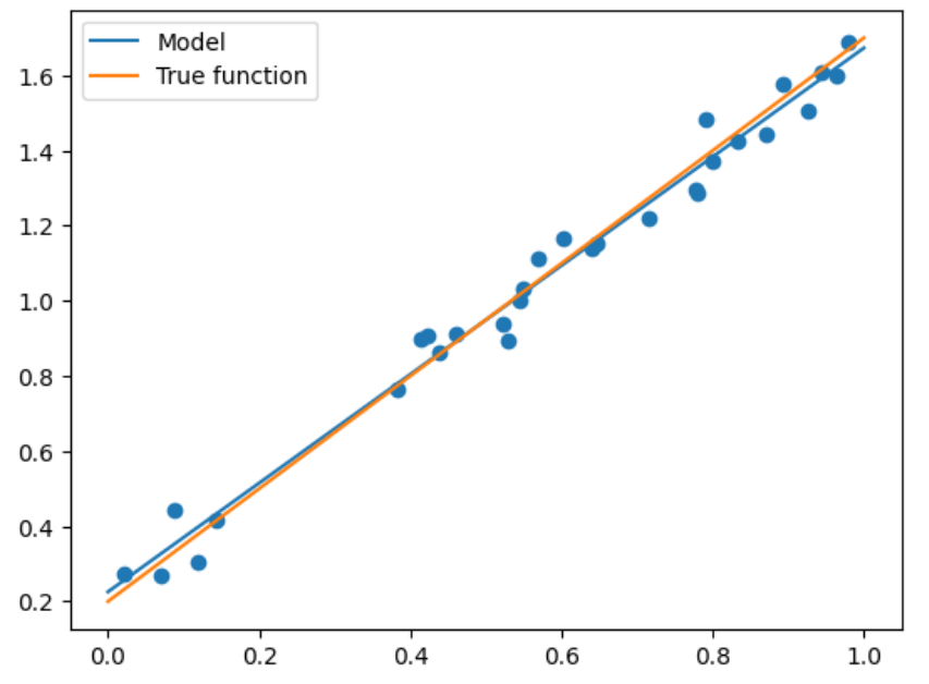
可以看到我们输出为1.44和0.22,还是很接近真实答案的,那么我们选取一批测试集来看看精度:
X_test = np.linspace(0,1,100)  # 0和1之间,产生100个等间距的
plt.plot(X_test, model.predict(X_test[:, np.newaxis]), label = "Model")  # 将拟合出来的散点画出
plt.plot(X_test, true_fun(X_test), label = "True function")  # 真实结果
plt.scatter(X_train, y_train)  # 画出训练集的点
plt.legend(loc="best")  # 将标签放在最合适的位置
plt.show()

上述情况是最简单的,但当出现更高维度时,我们就需要进行多项式回归才能够满足需求了。
多项式回归
具体实现
对于多项式回归,一般是利用线性回归求解(y=\sum_{i=1}^m b_i \times x^i),因此算法如下:
import numpy as np
import matplotlib.pyplot as plt
from sklearn.pipeline import Pipeline
from sklearn.preprocessing import PolynomialFeatures  # 导入能够计算多项式特征的类
from sklearn.linear_model import LinearRegression
from sklearn.model_selection import cross_val_score  # 交叉验证

def true_fun(X):  # 真实函数
    return np.cos(1.5 * np.pi * X)

np.random.seed(0)
n_samples = 30

X = np.sort(np.random.rand(n_samples))  # 随机采样后排序
y = true_fun(X) + np.random.randn(n_samples) * 0.1

degrees = [1, 4, 15] # 多项式最高次,我们分别用1次,4次和15次的多项式来尝试拟合
plt.figure(figsize=(14, 5))
for i in range(len(degrees)):
    ax = plt.subplot(1, len(degrees), i+1)  # 总共三个图,获取第i+1个图的图像柄
    plt.setp(ax, xticks = (), yticks = ())  # 这是 设置ax图中的属性
    polynomial_features = PolynomialFeatures(degree=degrees[i],include_bias=False)
    # 建立多项式回归的类,第一个参数就是多项式的最高次数,第二个是是否包含偏置
    linear_regression = LinearRegression()  # 线性回归
    pipeline = Pipeline([("polynomial_features", polynomial_features),
                         ("linear_regression", linear_regression)]) # 使用pipline串联模型
    pipeline.fit(X[:, np.newaxis], y)
    scores = cross_val_score(pipeline, X[:, np.newaxis], y, scoring="neg_mean_squared_error", cv=10)
    # 使用交叉验证,第一个参数为模型,第二个为输入,第三个为标签,第四个为误差计算方式,第五个为多少折
    X_test = np.linspace(0, 1, 100)
    plt.plot(X_test, pipeline.predict(X_test[:, np.newaxis]), label="Model")
    plt.plot(X_test, true_fun(X_test), label="True function")
    plt.scatter(X, y, edgecolor='b', s=20, label="Samples")
    plt.xlabel("x")
    plt.ylabel("y")
    plt.xlim((0, 1))
    plt.ylim((-2, 2))
    plt.legend(loc="best")
    plt.title("Degree {}\nMSE = {:.2e}(+/- {:.2e})".format(degrees[i], -scores.mean(), scores.std()))
plt.show()
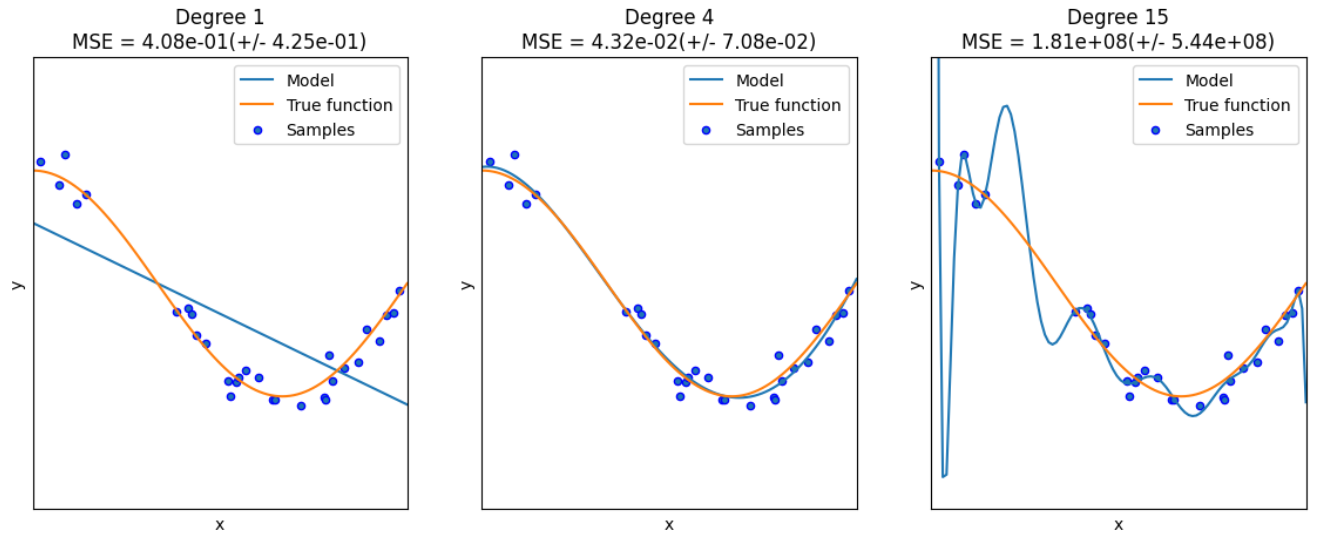
这里解释两个地方:
- PolynomialFeatures:这个类实际上是一个构造特征的类,因为我们原始的X是一个一维的向量,它多项式的次数为1,那我们希望构成一个多项式就需要拿X去计算(X^1,X^2,…,X^m)(这是一个变量的情况,如果是多个变量就会计算交叉乘),那么这个类就是实现这样的操作,构造成m个特征
- pipeline:这是方便我们的管道,它将各种模块加在一起让我们不用一步步去计算每一个模块,这里就是将PolynomialFeatures和线性回归模块加在一起,那我们将X传进去之后,就经过特征构造后就进行线性回归,因此 拟合管道即可。
在其中我们还用到了交叉验证的思路,这部分很常见就不多做解释了。
LogisticRegression
算法思想简述
对于逻辑回归大部分是面对二分类问题,给定数据(X={x_1,x_2,…,},Y={y_1,y_2,…,})
考虑二分类任务,那么其假设函数就是:
[h_{\theta}(x) = g(\theta^Tx)=g(w^Tx+b)=\frac{1}{1+e^{w^Tx+b}} ]
来表示为类别1或者类别0的概率。
那么其损失函数一般是采用极大似然估计法来定义:
[L(\theta)=\prod_{i=1}p(y_i=1\mid x_i)=h_{\theta}(x_1)(1-h_{\theta}(x))… ]
这里假设(y_1=1,y_2=0)。那么就是该函数最大化,化简可得:
[\theta^{*}=arg\min_{\theta}(-L(\theta))=arg\min_{\theta}-\ln(L(\theta))\ =\sum_{i=1}(-y_i\theta^Tx_i+\ln(1+e^{\theta^Tx_i})) ]
再利用梯度下降即可。
算法实现
下面为sklearn版本
import numpy as np
from sklearn.datasets import fetch_openml

mnist = fetch_openml("mnist_784")  # 数据
X, y = mnist['data'], mnist['target']
X_train = np.array(X[:60000], dtype = float)
y_train = np.array(y[:60000], dtype = float)
X_test = np.array(X[60000:], dtype = float)
y_test = np.array(y[60000:], dtype = float)  # 构造训练集和数据集
print(X_train.shape)
print(y_train.shape)
print(X_test.shape)
print(y_test.shape)
(60000, 784)
(60000,)
(10000, 784)
(10000,)
from sklearn.linear_model import LogisticRegression
clf = LogisticRegression(penalty='l1', solver='saga', tol=0.1)
第一个参数为惩罚项选择l1还是l2,tol是停止求解的条件,solver可以认为是求解器
clf.fit(X_train, y_train)
score = clf.score(X_test, y_test)
print("Test score with L1 penalty: %.4f" % score)
Test score with L1 penalty: 0.9245
这里我好奇的是逻辑回归面对的是二分类问题,可是这里我们直接给他多分类问题的数据集为何能够直接求解,查了一遍发现是类内部的优化帮你实现了这一过程。
以下为pytorch版本
from torch.utils.data import DataLoader
from torchvision import datasets
import torchvision
import torchvision.transforms as transforms
import matplotlib.pyplot as plt
from sklearn.linear_model import LogisticRegression
from sklearn.metrics import classification_report
import numpy as np
train_dataset = datasets.MNIST(root = p_parent_path+'/datasets/', train = True,transform = transforms.ToTensor(), download = False)
test_dataset = datasets.MNIST(root = p_parent_path+'/datasets/', train = False, transform = transforms.ToTensor(), download = False)
#加载数据集
batch_size = len(train_dataset)
train_loader = DataLoader(dataset=train_dataset, batch_size=batch_size, shuffle=True)
test_loader = DataLoader(dataset=test_dataset, batch_size=batch_size, shuffle=True)
数据加载器
X_train,y_train = next(iter(train_loader))
X_test,y_test = next(iter(test_loader))
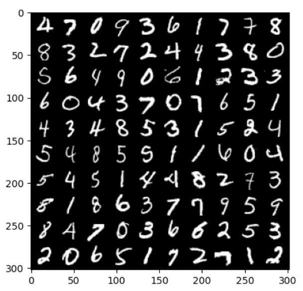
打印前100张图片
images, labels= X_train[:100], y_train[:100]
使用images生成宽度为10张图的网格大小
img = torchvision.utils.make_grid(images, nrow=10)
cv2.imshow()的格式是(size1,size1,channels),而img的格式是(channels,size1,size1),
所以需要使用.transpose()转换,将颜色通道数放至第三维
img = img.numpy().transpose(1,2,0)
print(images.shape)
print(labels.reshape(10,10))
print(img.shape)
plt.imshow(img)
plt.show()
torch.Size([100, 1, 28, 28])
tensor([[4, 7, 0, 9, 3, 6, 1, 7, 7, 8],
        [8, 3, 2, 7, 2, 4, 4, 3, 8, 0],
        [5, 6, 4, 9, 0, 6, 1, 2, 3, 3],
        [6, 0, 4, 3, 7, 0, 7, 6, 5, 1],
        [4, 3, 4, 8, 5, 3, 1, 5, 2, 4],
        [5, 4, 8, 5, 5, 1, 1, 6, 0, 4],
        [5, 4, 5, 1, 4, 4, 8, 2, 7, 3],
        [8, 1, 8, 6, 3, 7, 7, 9, 5, 9],
        [8, 4, 7, 0, 3, 6, 6, 2, 5, 3],
        [2, 0, 6, 5, 1, 7, 2, 7, 1, 2]])
(302, 302, 3)
X_train,y_train = X_train.cpu().numpy(),y_train.cpu().numpy() # tensor转为array形式)
X_test,y_test = X_test.cpu().numpy(),y_test.cpu().numpy() # tensor转为array形式)
X_train = X_train.reshape(X_train.shape[0],784)  # 展开成1维度的向量的形式,长度为28*28等于784
X_test = X_test.reshape(X_test.shape[0],784)
model = LogisticRegression(solver='lbfgs', max_iter = 400)
model.fit(X_train, y_train)
y_pred = model.predict(X_test)
print(classification_report(y_test, y_pred)) # 打印报告
precision    recall  f1-score   support

           0       0.50      0.75      0.60         4
           1       0.71      1.00      0.83        10
           2       0.79      0.85      0.81        13
           3       0.79      0.69      0.73        16
           4       0.83      0.91      0.87        11
           5       0.60      0.23      0.33        13
           6       1.00      1.00      1.00         5
           7       0.88      1.00      0.93         7
           8       0.67      0.83      0.74        12
           9       0.71      0.56      0.63         9

    accuracy                           0.75       100
   macro avg       0.75      0.78      0.75       100
weighted avg       0.74      0.75      0.73       100
Decision Tree
首先介绍一个数据集,鸢尾花(iris)数据集,数据集内包含 3 类共 150 条记录,每类各 50 个数据,每条记录都有 4 项特征:花萼长度、花萼宽度、花瓣长度、花瓣宽度,可以通过这4个特征预测鸢尾花卉属于(iris-setosa, iris-versicolour, iris-virginica)中的哪一品种。
import seaborn as sns
from pandas import plotting
import pandas as pd
import numpy as np
import matplotlib.pyplot as plt
from sklearn.tree import DecisionTreeClassifier
from sklearn.datasets import load_iris
from sklearn.model_selection import train_test_split
from sklearn import tree

加载数据集
data = load_iris()
转换成DataFrame的格式
df = pd.DataFrame(data.data, columns=data.feature_names)
df['Species'] = data.target  # 添加品种列
查看数据集信息
print(f"数据集信息:\n{df.info()}")
查看前5条数据
print(f"前5条数据:\n{df.head()}")
df.describe()
RangeIndex: 150 entries, 0 to 149
Data columns (total 5 columns):
# Column Non-Null Count Dtype
Original: https://www.cnblogs.com/FavoriteStar/p/16925556.html
Author: FavoriteStar
Title: 基于Sklearn机器学习代码实战
原创文章受到原创版权保护。转载请注明出处:https://www.johngo689.com/804565/
转载文章受原作者版权保护。转载请注明原作者出处!