

直方图(Histogram),一种数据统计层面的绘图方式。用一系列高低不等的柱子表示数据分布,横坐标表示数据划分区间,纵坐标可以表示落到各个区间内的频数/频率。使用 matplotlib.pyplot库中的 hist方法实现,先看函数的参数:官方link
matplotlib.pyplot.hist(x, bins=None, range=None, density=False, weights=None, cumulative=False, bottom=None, histtype='bar', align='mid', orientation='vertical', rwidth=None, log=False, color=None, label=None, stacked=False, *, data=None, **kwargs)
x是输入的数据,一般是一维数组,必填项。bins是数据划分的组数,可以根据实际情况自己设置,也可以默认适配。range需要tuple类型数据(x_min,x_max),表示bin的下界和上届,也可以默认。density当你需要纵轴显示频率时,将该参数设置为True。其中,内部是通过该公式计算的频率density = counts / (sum(counts) * np.diff(bins))np.sum(density * np.diff(bins)) == 1。如果stacked也是True,则直方图的总和归一化为 1。(尝试了一下,有些数据不知道为啥纵坐标会大于1)weights与x形状相同的权重数组。x中的每个值仅将其相关权重贡献给 bin 计数(而不是 1)。如果密度为True,则权重被归一化,因此密度在该范围内的积分保持为 1。
weights = np.array(p) / len(p)
n, bins, patches=plt.hist(p,weights=weights)
注意: normed该属性已经被官方弃用,显示频率分布就看上述两种方式是否符合你的要求。
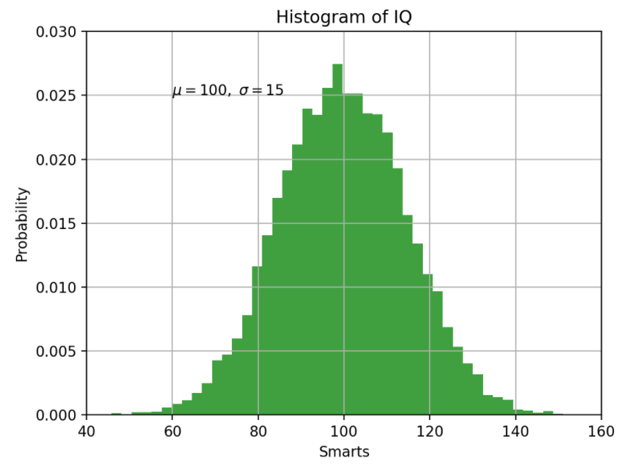
官方示例:
import numpy as np
import matplotlib.pyplot as plt

np.random.seed(19680801)

mu, sigma = 100, 15
x = mu + sigma * np.random.randn(10000)

n, bins, patches = plt.hist(x, 50, density=True, facecolor='g', alpha=0.75)

plt.xlabel('Smarts')
plt.ylabel('Probability')
plt.title('Histogram of IQ')
plt.text(60, .025, r'$\mu=100,\ \sigma=15$')
plt.xlim(40, 160)
plt.ylim(0, 0.03)
plt.grid(True)
plt.show()

Original: https://blog.csdn.net/qq_33866063/article/details/123111275
Author: 小卜妞~
Title: matplotlib直方图
原创文章受到原创版权保护。转载请注明出处:https://www.johngo689.com/770129/
转载文章受原作者版权保护。转载请注明原作者出处!