

多种分类以及模型评估
- 分类
* - 获取mnist数据集
- 获取训练数据和标签
- 数据标准化及数据集划分
- 训练二分类器
– - 多类分类器
–
分类
获取mnist数据集
from sklearn.datasets import fetch_openml
import numpy as np

mnist = fetch_openml('mnist_784', version=1)
mnist.keys()
运行结果:


其中:
DESCR:描述数据集
data:包含一个数组,每个实例一行,每个特征一列
target:包含一个带标记的数组
获取训练数据和标签
X, y = mnist['data'], mnist['target']
import matplotlib.pyplot as plt
import matplotlib as mpl

some_digit = np.array(X)[0]
some_digit_image = some_digit.reshape(28, 28)

plt.imshow(some_digit_image, cmap="binary")
plt.axis("off")
plt.show()
显示第0个图片

数据标准化及数据集划分
因为标签是字符型的,现在将字符型转换成无符号8位整型
y = y.astype(np.uint8)
mnist数据集已经分好了训练集(前60000)和测试集(后10000)这里直接分离就行
X_train, X_test, y_train, y_test = X[:60000], X[60000:], y[:60000], y[60000:]
训练二分类器
划分数据集
这里是将原来的0-9数据集按照5或非5进行划分
y_train_5 = (y_train == 5)
y_test_5 = (y_test == 5)
随机梯度下降分类
from sklearn.linear_model import SGDClassifier

sgd_clf = SGDClassifier(random_state=42)
sgd_clf.fit(X_train, y_train_5)
sgd_clf.predict([some_digit])
运行结果:
性能测试
使用交叉验证测量准确率
k折分层抽样:
from sklearn.model_selection import StratifiedKFold
from sklearn.base import clone

skfolds = StratifiedKFold(n_splits=3)

for train_index, test_index in skfolds.split(X_train, y_train_5):
    clone_clf = clone(sgd_clf)

    X_train_flods = np.array(X_train)[train_index]
    y_train_flods = y_train_5[train_index]

    X_test_flods = np.array(X_train)[test_index]
    y_test_flods = y_train_5[test_index]

    clone_clf.fit(X_train_flods, y_train_flods)
    y_pred = clone_clf.predict(X_test_flods)
    n_correct = sum(y_pred == y_test_flods)
    print(n_correct / len(y_pred))
运行结果:

交叉验证:
from sklearn.model_selection import cross_val_score
cross_val_score(sgd_clf, X_train, y_train_5, cv=3, scoring="accuracy")
运行结果:

傻瓜版分类器
from sklearn.base import BaseEstimator

class Never5Classifier(BaseEstimator):
    def fit(self, X, y=None):
        return self
    def predict(self, X):
        return np.zeros((len(X), 1), dtype=bool)

never_5_clf = Never5Classifier()
cross_val_score(never_5_clf, X_train, y_train_5, cv=3, scoring="accuracy")
运行结果:

因为5的数据为占全部数据的1/10,所以随机的结果也很好,但是这种很好的表现是一种虚假的表现。
混淆矩阵
随机梯度下降分类器对应的混淆矩阵
计算混淆矩阵需要有预测值才能和实际目标比较,这里暂时不使用测试集,所以使用cross_val_predict替代
from sklearn.model_selection import cross_val_predict
from sklearn.metrics import confusion_matrix
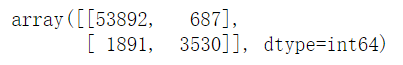
y_train_pred = cross_val_predict(sgd_clf, X_train, y_train_5, cv=3)
confusion_matrix(y_train_5, y_train_pred)
运行结果:
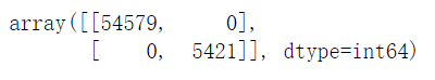
混淆矩阵最佳状态
y_train_perfect_predictions = y_train_5
confusion_matrix(y_train_5, y_train_perfect_predictions)
运行结果:
精度和召回率
精度 = TP(真正类[判别为正类的真正的正类]) / (TP + FP(假正类[判断为正类的不是正类])) 判出来的真正的正类和真正的正类的比
召回率 = TP / (TP(真正类) + FN(假负类)) 判出来的真正的正类和所有被判为正类的比
from sklearn.metrics import precision_score, recall_score

precision_score(y_train_5, y_train_pred)
运行结果:
recall_score(y_train_5, y_train_pred)
运行结果:

从上面可以看出来,当一个数据是5时,有precision_score的概率是准确的, 只有recall_score的5被检测出来
将精度和召回率组合成单一的指标F1分数,F1分数是精度和召回率的谐波平均值,谐波平均值会给予低的值更高的权重,只有召回率和精度都很高时分类器才能得到较高的F1分数
F1 = 2 / (1/精度 + 1/召回率) = 2 * 精度 * 召回率 /(精度 + 召回率) = TP/(TP+(FN+FP)/2)
from sklearn.metrics import f1_score

f1_score(y_train_5, y_train_pred)
运行结果:
F1对于精度和召回率相近的分类器有利
精度/召回率权衡
提高阈值精度提升,降低阈值会增加召回率降低精度
y_scores= sgd_clf.decision_function([some_digit])
y_scores
运行结果:

阈值为0的情况
threshold = 0
y_some_digit_pred = (y_scores > threshold)
y_some_digit_pred
运行结果:
阈值为8000的情况
threshold = 8000
y_some_digit_pred = (y_scores > threshold)
y_some_digit_pred
运行结果:
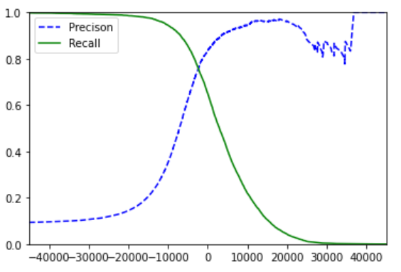
阈值对精度和召回率影响变化图像
y_scores = cross_val_predict(sgd_clf, X_train, y_train_5, cv=3, method="decision_function")
from sklearn.metrics import precision_recall_curve

precisions, recalls, thresholds = precision_recall_curve(y_train_5, y_scores)
def plot_precision_recall_vs_threshold(precisions, recalls, thresholds):
    plt.plot(thresholds, precisions[:-1], "b--", label="Precison")
    plt.plot(thresholds, recalls[:-1], "g-", label="Recall")
    plt.xlim(-45000, 45000)
    plt.ylim(0, 1)
    plt.legend()

plot_precision_recall_vs_threshold(precisions, recalls, thresholds)
plt.show()
确定阈值
假设现在要将精度设为90%,首先查阈值
np.argmax(precisions > 0.9)
运行结果:

threshold_90_precision = thresholds[np.argmax(precisions >= 0.90)]
threshold_90_precision
y_train_pred_90 = (y_scores >= threshold_90_precision)
precision_score(y_train_5, y_train_pred_90)
recall_score(y_train_5, y_train_pred_90)
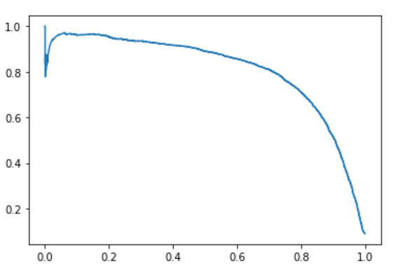
plt.plot(recalls, precisions)
plt.show()
ROC曲线
受试者工作特征曲线(简称ROC),描绘的是真正类率(召回率)和假正类率(FPR),FPR是被错误分为正类的负类实例的比值,等于1-真负类率(TNR)
from sklearn.metrics import roc_curve

fpr, tpr, thresholds = roc_curve(y_train_5, y_scores)
def plot_roc_curve(fpr, tpr, label=None):
    plt.plot(fpr, tpr, linewidth=2, label=label)
    plt.plot([0, 1], [0, 1], 'k--')

plot_roc_curve(fpr, tpr)
plt.show()
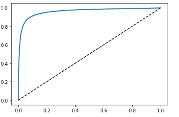
这里面临一个折中权衡,召回率(TPR)越高,分类器产生的假正类(FPR)就越多,虚线表示纯随机分类器的ROC曲线,一个优秀的分类器应该离这个线越远越好
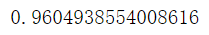
from sklearn.metrics import roc_auc_score

roc_auc_score(y_train_5, y_scores)
由于ROC曲线与精度/召回率(PR)曲线非常相似,当正类非常少见或者更关注假正类而不是假负类时,应该选择PR曲线,反之是ROC曲线
跟负类(非5)相比,正类(数字5)的数量真的很少,PR曲线清楚的说明分类器还有改进的空间
现在来训练一个随机森林分类器并比较他和随机梯度下降分类器的ROC曲线和ROC AUC分数
from sklearn.ensemble import RandomForestClassifier

forest_clf = RandomForestClassifier(random_state=42)
y_probas_forest = cross_val_predict(forest_clf, X_train, y_train_5, cv=3, method="predict_proba")
roc_curve需要标签和分数,这里直接使用正类的概率作为分数值
y_probas_forest
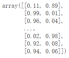
y_score_forest = y_probas_forest[:, 1]
fpr_forest, tpr_forest, thresholds_forest = roc_curve(y_train_5, y_score_forest)
plt.plot(fpr, tpr,"b:", label="SGD")
plot_roc_curve(fpr_forest, tpr_forest, "Random Forest")
plt.legend(loc="lower right")
plt.show()
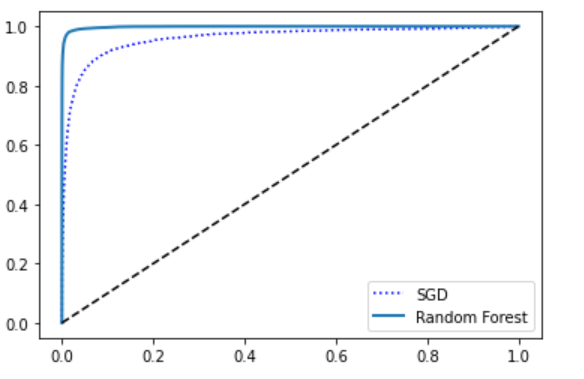
比较ROC曲线,随机森林优于随机梯度下降
roc_auc_score(y_train_5, y_score_forest)
测试精度和召回率
precision_score(y_train_5, y_score_forest > 0.5)
recall_score(y_train_5, y_score_forest > 0.5)
多类分类器
OvR与OvO
OvR策略:一对剩余 ;OvO策略:一对一
scikit-Learn 可以检测尝试使用二分类算法进行多类分类任务,会根据情况自动运行OvR,OvO, 下面用sklearn.svm.SVC类试试SVM分类器(SVM是支持向量机,这里就是拿来举个例子,后面的章节还会具体介绍)
from sklearn.svm import SVC

svm_clf = SVC()
svm_clf.fit(X_train, y_train)
svm_clf.predict([some_digit])
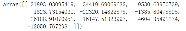
在内部实际上训练了45个二元分类器,为了测试是否是这样,调用decision_function(),会返回10个分数
some_digit_scores = svm_clf.decision_function([some_digit])
some_digit_scores

from sklearn.multiclass import OneVsRestClassifier
ovr_clf = OneVsRestClassifier(SVC())
ovr_clf.fit(X_train, y_train)
ovr_clf.predict([some_digit])
随机梯度下降和随机森林
sgd_clf.fit(X_train, y_train)
sgd_clf.predict([some_digit])
sgd_clf.decision_function([some_digit])
cross_val_score(sgd_clf, X_train, y_train, cv=3, scoring="accuracy")

from sklearn.preprocessing import StandardScaler

scaler = StandardScaler()
X_train_scaled = scaler.fit_transform(X_train.astype(np.float64))
cross_val_score(sgd_clf, X_train_scaled, y_train, cv=3, scoring="accuracy")

误差分析
假设现在已经有了一个有潜力的模型,现在希望找到一些方法对其进一步改进,其中的一种方法就是分析其错误类型(误判的类型,即为什么会被误判)
y_train_pred = cross_val_predict(sgd_clf, X_train_scaled, y_train, cv=3)
conf_mx = confusion_matrix(y_train, y_train_pred)
conf_mx
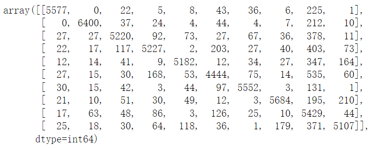
由于数字较多,并且不够直观,这里使用matshow(这个的作用是将矩阵绘制成图像,注意区分他和热力图的区别)查看混淆矩阵的图像表示
plt.matshow(conf_mx, cmap=plt.cm.gray)
plt.show()
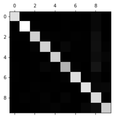
大多数图片都在对角线上,说明基本上是被正确分类了(一个好的分类器的对角线是比较亮的)
row_sums = conf_mx.sum(axis=1, keepdims=True)
norm_conf_mx = conf_mx / row_sums
用0填充对角线,只保留错误,重新绘制结果(实际上就是降低亮度,来突出误判的亮度)
np.fill_diagonal(norm_conf_mx, 0)
plt.matshow(norm_conf_mx, cmap=plt.cm.gray)
plt.show()
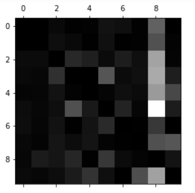
可以看到8的这个类别里面错误的分类要多,后续的优化可以针对8来进行(书中写的是搜集更多像8的数据,或者用算法计算闭环)
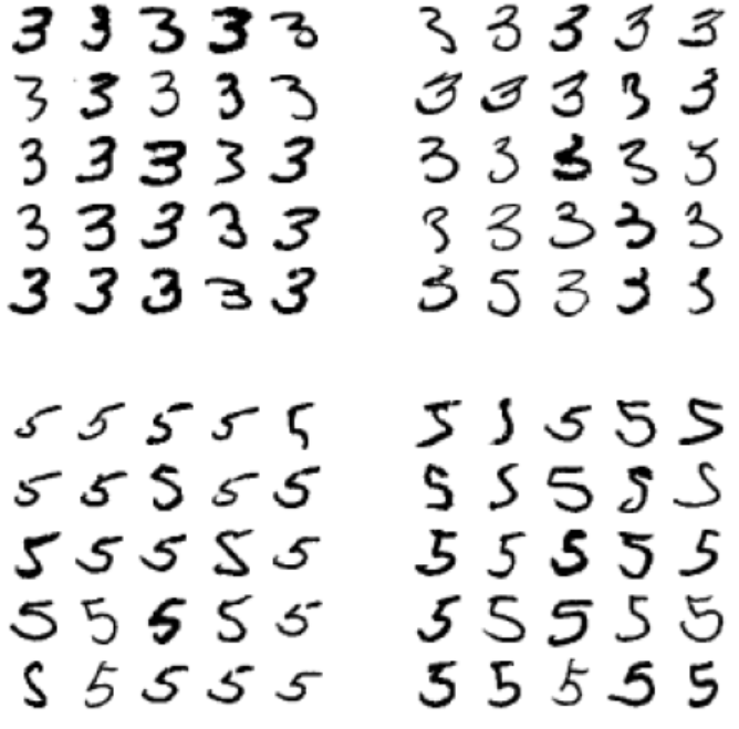
3和5误判的情况
def plot_digits(instances, images_per_row=10, **options):
    size = 28
    images_per_row = min(len(instances), images_per_row)
    images = [np.array(instances.iloc[i]).reshape(size, size) for i in range(instances.shape[0])]

    if images_per_row == 0:
       images_per_row = 0.1

    n_rows = (len(instances) - 1) // images_per_row + 1
    row_images = []
    n_empty = n_rows * images_per_row - len(instances)
    images.append(np.zeros((size, size * n_empty)))
    for row in range(n_rows):
        rimages = images[row * images_per_row : (row + 1) * images_per_row]
        row_images.append(np.concatenate(rimages, axis=1))
    image = np.concatenate(row_images, axis=0)
    plt.imshow(image, cmap = plt.cm.binary, **options)
    plt.axis("off")

cl_a, cl_b = 3, 5
X_aa = X_train[(y_train == cl_a) & (y_train_pred == cl_a)]
X_ab = X_train[(y_train == cl_a) & (y_train_pred == cl_b)]
X_bb = X_train[(y_train == cl_b) & (y_train_pred == cl_b)]
X_ba = X_train[(y_train == cl_b) & (y_train_pred == cl_a)]

plt.figure(figsize=(8, 8))
plt.subplot(221);plot_digits(X_aa[:25], images_per_row=5)
plt.subplot(222);plot_digits(X_ab[:25], images_per_row=5)
plt.subplot(223);plot_digits(X_bb[:25], images_per_row=5)
plt.subplot(224);plot_digits(X_ba[:25], images_per_row=5)
plt.show()
多标签分类
输出多个标签的分类器(之前介绍的分类器的结果都只有一个标签)
from sklearn.neighbors import KNeighborsClassifier
y_train_large = (y_train >= 7)
y_train_odd = (y_train % 2 == 1)
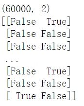
y_multilabel = np.c_[y_train_large, y_train_odd]
print(y_multilabel.shape)
print(y_multilabel)
knn_clf = KNeighborsClassifier()
knn_clf.fit(X_train, y_multilabel)
训练出来的模型预测结果包括两个标签,一个判断是不是大数,一个判断是不是奇数(这种方式不推荐,因为增加了模型的运算量,会影响精度,一般是先预测出数字,再判断是不是大数和奇数)
knn_clf.predict([some_digit])
y_train_knn_pred = cross_val_predict(knn_clf, X_train, y_multilabel, cv=3)
f1_score(y_multilabel, y_train_knn_pred, average="macro")
多输出分类
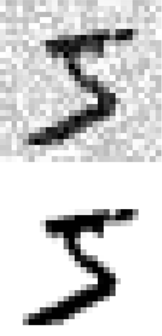
大体上和多标签分类相似,是多标签分类的泛化,下面用图片降噪为例说明多输出分类
noise = np.random.randint(0, 100, (len(X_train), 784))
X_train_mod = X_train + noise
noise = np.random.randint(0, 100, (len(X_test), 784))
X_test_mod = X_test + noise
y_train_mod = X_train
y_test_mod = X_test
some_index = 1
plt.imshow(np.array(X_train_mod[some_index-1:some_index]).reshape((28, 28)), cmap="binary")
plt.axis("off")
plt.show()
plt.imshow(np.array(y_train_mod[some_index-1:some_index]).reshape((28, 28)), cmap="binary")
plt.axis("off")
plt.show()
knn_clf.fit(X_train_mod, y_train_mod)
clean_digit = knn_clf.predict(X_test_mod[some_index-1:some_index])
plt.imshow(np.array(X_test_mod[some_index-1:some_index]).reshape(28, 28), cmap="binary")
plt.axis("off")
plt.show()
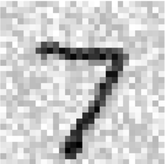
plt.imshow(np.array(clean_digit).reshape(28, 28), cmap="binary")
plt.axis("off")
plt.show()

Original: https://blog.csdn.net/DuLNode/article/details/120144085
Author: 艾醒(AiXing-w)
Title: 多种分类以及模型评估
原创文章受到原创版权保护。转载请注明出处:https://www.johngo689.com/767754/
转载文章受原作者版权保护。转载请注明原作者出处!