

文章目录
数据分析 第七讲 pandas练习 数据的合并和分组聚合


; 一、pandas-DataFrame
练习1
对于这一组电影数据,如果我们想runtime(电影时长)的分布情况,应该如何呈现数据?
数据分析
import pandas as pd
from matplotlib import pyplot as plt
import matplotlib
font = {
'family':'SimHei',
'weight':'bold',
'size':12
}
matplotlib.rc("font", **font)
file_path = './IMDB-Movie-Data.csv'
df = pd.read_csv(file_path)

'''

RangeIndex: 1000 entries, 0 to 999
Data columns (total 12 columns):
 #   Column              Non-Null Count  Dtype
 0   Brand           25600 non-null  object
 1   Store Number    25600 non-null  object
 2   Store Name      25600 non-null  object
 3   Ownership Type  25600 non-null  object
 4   Street Address  25598 non-null  object
 5   City            25585 non-null  object
 6   State/Province  25600 non-null  object
 7   Country         25600 non-null  object
 8   Postcode        24078 non-null  object
 9   Phone Number    18739 non-null  object
 10  Timezone        25600 non-null  object
 11  Longitude       25599 non-null  float64
 12  Latitude        25599 non-null  float64
dtypes: float64(2), object(11)
memory usage: 2.5+ MB
None'''
print(df.head())
'''
       Brand  Store Number  ... Longitude Latitude
0  Starbucks  47370-257954  ...      1.53    42.51
1  Starbucks  22331-212325  ...     55.47    25.42
2  Starbucks  47089-256771  ...     55.47    25.39
3  Starbucks  22126-218024  ...     54.38    24.48
4  Starbucks  17127-178586  ...     54.54    24.51
'''
pd.set_option('display.max_rows', 10)
pd.set_option('display.max_columns', 13)
print(df)
'''
                        City State/Province Country Postcode  Phone Number  \
0           Andorra la Vella              7      AD    AD500     376818720
1                      Ajman             AJ      AE      NaN           NaN
2                      Ajman             AJ      AE      NaN           NaN
3                  Abu Dhabi             AZ      AE      NaN           NaN
4                  Abu Dhabi             AZ      AE      NaN           NaN
...                      ...            ...     ...      ...           ...

25595  Thành Phố Hồ Chí Minh             SG      VN    70000  08 3824 4668
25596  Thành Phố Hồ Chí Minh             SG      VN    70000  08 5413 8292
25597           Johannesburg             GT      ZA     2194   27873500159
25598                 Menlyn             GT      ZA      181           NaN
25599                Midrand             GT      ZA     1682   27873500215

                             Timezone  Longitude  Latitude
0             GMT+1:00 Europe/Andorra       1.53     42.51
1                GMT+04:00 Asia/Dubai      55.47     25.42
2                GMT+04:00 Asia/Dubai      55.47     25.39
3                GMT+04:00 Asia/Dubai      54.38     24.48
4                GMT+04:00 Asia/Dubai      54.54     24.51
...                               ...        ...       ...

25595          GMT+000000 Asia/Saigon     106.70     10.78
25596          GMT+000000 Asia/Saigon     106.71     10.72
25597  GMT+000000 Africa/Johannesburg      28.04    -26.15
25598  GMT+000000 Africa/Johannesburg      28.28    -25.79
25599  GMT+000000 Africa/Johannesburg      28.11    -26.02

[25600 rows x 13 columns]
'''
grouped = df.groupby(by='Country').count()['Brand']
print(type(grouped))
print(grouped)
'''
AD        1
AE      144
AR      108
AT       18
AU       22
      ...

TT        3
TW      394
US    13608
VN       25
ZA        3
Name: Brand, Length: 73, dtype: int64'''
us_count = grouped['US']
print(us_count)
cn_count = grouped['CN']
print(cn_count)
print("美国的星巴克总数位%s,中国的星巴克为%s" % (us_count, cn_count))
'''美国的星巴克总数位13608,中国的星巴克为2734'''

china_data = df[df['Country'] == 'CN']
print(china_data)
'''
          Brand  Store Number           Store Name Ownership Type  \
2091  Starbucks  22901-225145            北京西站第一咖啡店  Company Owned
2092  Starbucks  32320-116537              北京华宇时尚店  Company Owned
2093  Starbucks  32447-132306           北京蓝色港湾圣拉娜店  Company Owned
2094  Starbucks  17477-161286           北京太阳宫凯德嘉茂店  Company Owned
2095  Starbucks  24520-237564              北京东三环北店  Company Owned
...         ...           ...                  ...            ...

4820  Starbucks  17872-186929                Sands       Licensed
4821  Starbucks  24126-235784              Wynn II       Licensed
4822  Starbucks  28490-242269      Wynn Palace BOH       Licensed
4823  Starbucks  22210-218665  Sands Cotai Central       Licensed
4824  Starbucks  17108-179449          One Central       Licensed

                                         Street Address   City State/Province  \
2091                          丰台区, 北京西站通廊7-1号, 中关村南大街2号    北京市             11
2092          海淀区, 数码大厦B座华宇时尚购物中心内, 蓝色港湾国际商区1座C1-3单元首层、    北京市             11
2093                朝阳区朝阳公园路6号, 二层C1-3单元及二层阳台, 太阳宫中路12号    北京市             11
2094                  朝阳区, 太阳宫凯德嘉茂一层01-44/45号, 东三环北路27号    北京市             11
2095                      朝阳区, 嘉铭中心大厦A座B1层024商铺, 金融大街7号    北京市             11
...                                                 ...    ...            ...

4820  Portion of Shop 04, Ground Floor, Sands, Largo...  Macau             92
4821             Wynn Macau, Rua Cidada de Sintra, NAPE  Macau             92
4822       Employee Entrance Outlet, Wynn Cotai, Resort  Macau             92
4823  Shop K201 & K202, Level 02, Parcela 5&6, Estra...  Macau             92
4824                       Promenade Rd, Open Area, 2/F  Macau             92

     Country Postcode   Phone Number                Timezone  Longitude  \
2091      CN   100073            NaN  GMT+08:00 Asia/Beijing     116.32
2092      CN   100086   010-51626616  GMT+08:00 Asia/Beijing     116.32
2093      CN   100020   010-59056343  GMT+08:00 Asia/Beijing     116.47
2094      CN   100028   010-84150945  GMT+08:00 Asia/Beijing     116.45
2095      CN      NaN            NaN  GMT+08:00 Asia/Beijing     116.46
...      ...      ...            ...                     ...        ...

4820      CN      NaN  (853)28782773  GMT+08:00 Asia/Beijing     113.55
4821      CN      NaN    85328723516  GMT+08:00 Asia/Beijing     113.55
4822      CN      NaN            NaN  GMT+08:00 Asia/Beijing     113.54
4823      CN      NaN    85328853439  GMT+08:00 Asia/Beijing     113.56
4824      CN      NaN            NaN  GMT+08:00 Asia/Beijing     113.55

      Latitude
2091     39.90
2092     39.97
2093     39.95
2094     39.97
2095     39.93
...        ...

4820     22.19
4821     22.19
4822     22.20
4823     22.15
4824     22.19

[2734 rows x 13 columns]
'''
china_province_data = china_data.groupby(by='State/Province').count()
print(china_province_data['Brand'])
'''
State/Province
11    236
12     58
13     24
14      8
15      8
     ...

62      3
63      3
64      2
91    162
92     13
Name: Brand, Length: 31, dtype: int64'''
- DataFrameGroupBy对象方法
方法 说明
count 分组中非NA值的数量
sum 非NA值的和
mean 非NA值的平均值
min,max 非NA值的最小值和最大值
4.索引和复合索引
- 简单的索引操作: t.index
- 指定index: t.index = [‘a’,’b’,’c’]
- 重新设置index : t.reindex([“a”,”e”])
- 指定某一列作为index : t.set_index(“M”,drop=False)
- 返回index的唯一值: t.set_index(“M”).index.unique()
-
设置两个索引的时候会是什么样子呢?
-
示例
import numpy as np
import pandas as pd

t1 = pd.DataFrame(np.arange(12).reshape(3, 4), index=list('ABC'), columns=list('WXYZ'))
print(t1)
'''
   W  X   Y   Z
A  0  1   2   3
B  4  5   6   7
C  8  9  10  11'''
print(t1.index)

print(t1.reindex(['a','e']))
'''
    W   X   Y   Z
a NaN NaN NaN NaN
e NaN NaN NaN NaN'''
print(t1.reindex(['A','e']))
'''
     W    X    Y    Z
A  0.0  1.0  2.0  3.0
e  NaN  NaN  NaN  NaN'''

print(t1.set_index('W'))
'''
   X   Y   Z
W
0  1   2   3
4  5   6   7
8  9  10  11'''
print(t1.set_index('W',drop=False))
'''
   W  X   Y   Z
W
0  0  1   2   3
4  4  5   6   7
8  8  9  10  11'''

print(t1.set_index('W').index)
'''Int64Index([0, 4, 8], dtype='int64', name='W')'''
print(t1.set_index('W').index.unique())
'''Int64Index([0, 4, 8], dtype='int64', name='W')'''
t1.loc['B','W'] = 8
print(t1)
'''
   W  X   Y   Z
A  0  1   2   3
B  8  5   6   7
C  8  9  10  11'''
print(t1.set_index('W').index.unique())
'''Int64Index([0, 8], dtype='int64', name='W')'''

t2 = pd.DataFrame(np.arange(12).reshape(3, 4), index=list('ABC'), columns=list('WXYZ'))
print(t2)
'''
   W  X   Y   Z
A  0  1   2   3
B  4  5   6   7
C  8  9  10  11'''
print(t2.set_index(['W','X']))
'''
      Y   Z
W X
0 1   2   3
4 5   6   7
8 9  10  11'''
print(type(t2.set_index(['W','X'])))
Series复合索引
a = pd.DataFrame({‘a’: range(7),’b’: range(7, 0, -1),’c’: [‘one’,’one’,’one’,’two’,’two’,’two’, ‘two’],’d’:
list(“hjklmno”)})
设置c,d为索引
import numpy as np
import pandas as pd

a = pd.DataFrame({'a': range(7), 'b': range(7, 0, -1), 'c': ['one', 'one', 'one', 'two', 'two', 'two', 'two'], 'd':
    list("hjklmno")})
print(type(a))
print(a)
'''
   a  b    c  d
0  0  7  one  h
1  1  6  one  j
2  2  5  one  k
3  3  4  two  l
4  4  3  two  m
5  5  2  two  n
6  6  1  two  o'''
b = a.set_index(['c','d'])
print(b)
'''
       a  b
c   d
one h  0  7
    j  1  6
    k  2  5
two l  3  4
    m  4  3
    n  5  2
    o  6  1
'''
print(b.loc['one'])
'''
   a  b
d
h  0  7
j  1  6
k  2  5'''
print(b.loc['one'].loc['j'])
'''
a    1
b    6
Name: j, dtype: int64'''
print(b.loc['one'].loc['j']['a'])
c = b['a']
print(type(c))
print(c)
'''
c    d
one  h    0
     j    1
     k    2
two  l    3
     m    4
     n    5
     o    6
Name: a, dtype: int64'''
print(c['one']['j'])
print(c['one','j'])
设置d,c为索引
import numpy as np
import pandas as pd

a = pd.DataFrame({'a': range(7), 'b': range(7, 0, -1), 'c': ['one', 'one', 'one', 'two', 'two', 'two', 'two'], 'd':
    list("hjklmno")})
print(type(a))
print(a)
'''
   a  b    c  d
0  0  7  one  h
1  1  6  one  j
2  2  5  one  k
3  3  4  two  l
4  4  3  two  m
5  5  2  two  n
6  6  1  two  o'''
b = a.set_index(['d','c'])
print(b)
'''
       a  b
d c
h one  0  7
j one  1  6
k one  2  5
l two  3  4
m two  4  3
n two  5  2
o two  6  1
'''
print(b.loc['j'])
'''
     a  b
c
one  1  6'''
print(b.loc['j'].loc['one'])
'''
a    1
b    6
Name: one, dtype: int64'''
print(b.loc['j'].loc['one']['a'])
print(b.loc['j'].loc['one','a'])

print(b.swaplevel())
'''
       a  b
c   d
one h  0  7
    j  1  6
    k  2  5
two l  3  4
    m  4  3
    n  5  2
    o  6  1'''
DateFrame复合索引
import numpy as np
import pandas as pd

a = pd.DataFrame({'a': range(7), 'b': range(7, 0, -1), 'c': ['one', 'one', 'one', 'two', 'two', 'two', 'two'], 'd':
    list("hjklmno")})
print(type(a))
print(a)
'''
   a  b    c  d
0  0  7  one  h
1  1  6  one  j
2  2  5  one  k
3  3  4  two  l
4  4  3  two  m
5  5  2  two  n
6  6  1  two  o'''
b = a.set_index(['c','d'])
print(b)
'''
       a  b
c   d
one h  0  7
    j  1  6
    k  2  5
two l  3  4
    m  4  3
    n  5  2
    o  6  1
'''

print(b.loc['one'].loc['j','b'])

print(b.swaplevel().loc['j'].loc['one','b'])
5.练习
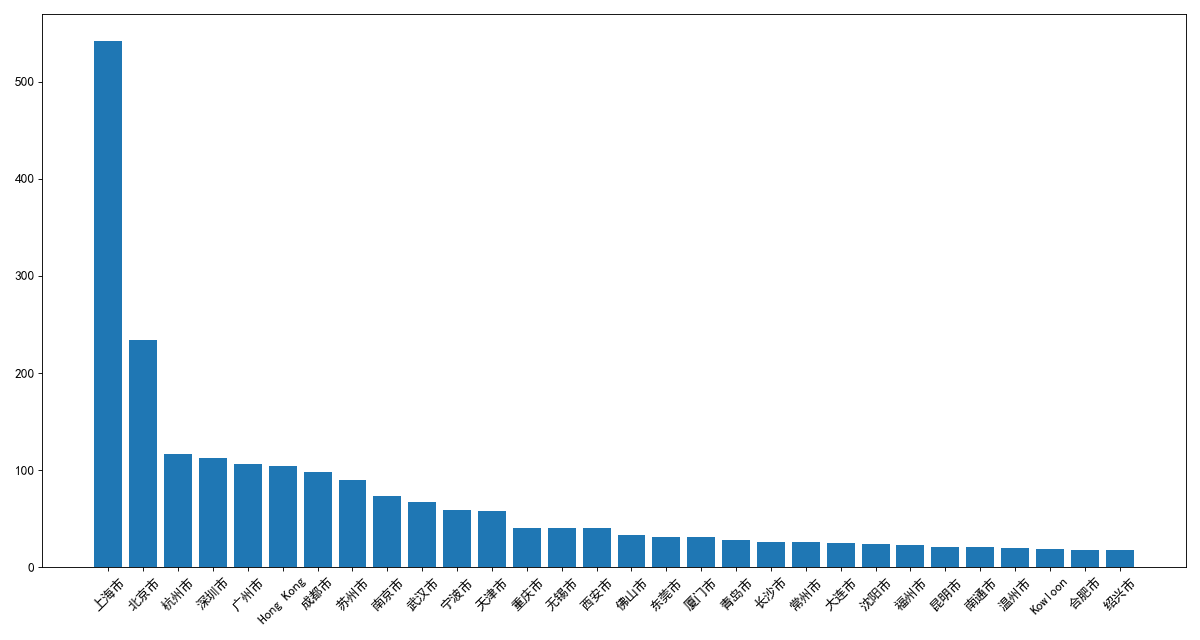
1.使用matplotlib呈现出店铺总数排名前10的国家
import numpy as np
import pandas as pd
from matplotlib import pyplot as plt

file_path = './starbucks_store_worldwide.csv'
df = pd.read_csv(file_path)
print(df.info())
'''

RangeIndex: 25600 entries, 0 to 25599
Data columns (total 13 columns):
 #   Column          Non-Null Count  Dtype
 0   Brand           25600 non-null  object
 1   Store Number    25600 non-null  object
 2   Store Name      25600 non-null  object
 3   Ownership Type  25600 non-null  object
 4   Street Address  25598 non-null  object
 5   City            25585 non-null  object
 6   State/Province  25600 non-null  object
 7   Country         25600 non-null  object
 8   Postcode        24078 non-null  object
 9   Phone Number    18739 non-null  object
 10  Timezone        25600 non-null  object
 11  Longitude       25599 non-null  float64
 12  Latitude        25599 non-null  float64
dtypes: float64(2), object(11)
memory usage: 2.5+ MB
None'''
df = df[df['Country'] == 'CN']

'''
          Brand  Store Number  ... Longitude Latitude
2091  Starbucks  22901-225145  ...    116.32    39.90
2092  Starbucks  32320-116537  ...    116.32    39.97
2093  Starbucks  32447-132306  ...    116.47    39.95

[3 rows x 13 columns]'''
data = df.groupby(by='City').count()['Brand'].sort_values(ascending=False)[0:30]
x = data.index
y = data.values

plt.figure(figsize=(15, 8), dpi=80)

plt.bar(x, y)

plt.xticks(rotation=45)
plt.show()
三、pandas中的时间序列
1.时间范围
时间范围
pd.date_range(start=None, end=None, periods=None, freq=’D’)
periods 时间范围的个数
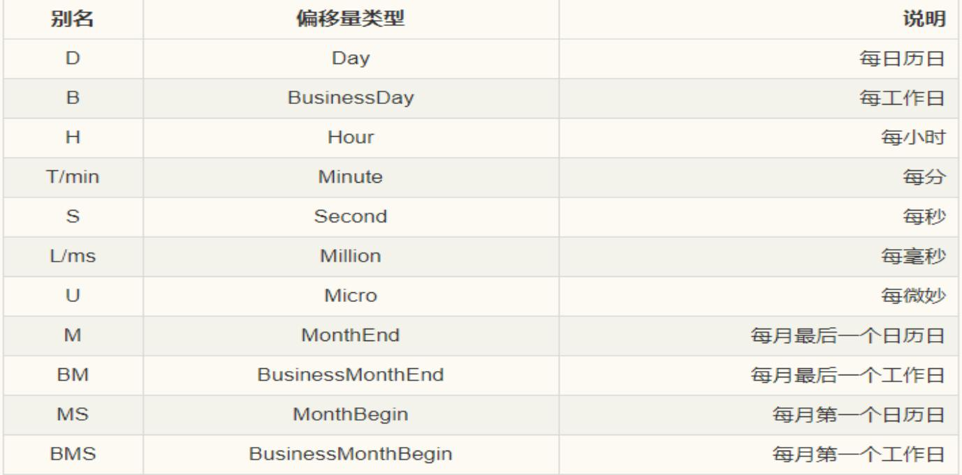
freq 频率,以天为单位还是以月为单位
关于频率的更多缩写
- 示例
import pandas as pd

d = pd.date_range(start='20210101', end='20210201')
print(d)
'''DatetimeIndex(['2021-01-01', '2021-01-02', '2021-01-03', '2021-01-04',
               '2021-01-05', '2021-01-06', '2021-01-07', '2021-01-08',
               '2021-01-09', '2021-01-10', '2021-01-11', '2021-01-12',
               '2021-01-13', '2021-01-14', '2021-01-15', '2021-01-16',
               '2021-01-17', '2021-01-18', '2021-01-19', '2021-01-20',
               '2021-01-21', '2021-01-22', '2021-01-23', '2021-01-24',
               '2021-01-25', '2021-01-26', '2021-01-27', '2021-01-28',
               '2021-01-29', '2021-01-30', '2021-01-31', '2021-02-01'],
              dtype='datetime64[ns]', freq='D')'''
m = pd.date_range(start='20210101', end='20211231',freq='M')
print(m)
'''
DatetimeIndex(['2021-01-31', '2021-02-28', '2021-03-31', '2021-04-30',
               '2021-05-31', '2021-06-30', '2021-07-31', '2021-08-31',
               '2021-09-30', '2021-10-31', '2021-11-30', '2021-12-31'],
              dtype='datetime64[ns]', freq='M')'''
d10 = pd.date_range(start='20210101', end='20210201',freq='10D')
print(d10)
'''
DatetimeIndex(['2021-01-01', '2021-01-11', '2021-01-21', '2021-01-31'], dtype='datetime64[ns]', freq='10D')'''
d3 = pd.date_range(start='20210101', end='20210201',freq='3D')
print(d3)
'''
DatetimeIndex(['2021-01-01', '2021-01-04', '2021-01-07', '2021-01-10',
               '2021-01-13', '2021-01-16', '2021-01-19', '2021-01-22',
               '2021-01-25', '2021-01-28', '2021-01-31'],
              dtype='datetime64[ns]', freq='3D')'''
d3 = pd.date_range(start='20210101', periods=5, freq='3D')
print(d3)
'''
DatetimeIndex(['2021-01-01', '2021-01-04', '2021-01-07', '2021-01-10',
               '2021-01-13'],
              dtype='datetime64[ns]', freq='3D')'''
2.DataFrame中使用时间序列
index=pd.date_range(“20190101”,periods=10)
df = pd.DataFrame(np.arange(10),index=index) 作为行索引
df = pd.DataFrame(np.arange(10).reshape(1,10),columns=index) 作为列索引
- 示例
import pandas as pd
import numpy as np

dindex = pd.date_range(start='20210101', periods=10)
df = pd.DataFrame(np.arange(10),index=dindex)
print(df)
'''
            0
2021-01-01  0
2021-01-02  1
2021-01-03  2
2021-01-04  3
2021-01-05  4
2021-01-06  5
2021-01-07  6
2021-01-08  7
2021-01-09  8
2021-01-10  9
'''

d_index = pd.date_range(start='20210101', periods=10)
df1 = pd.DataFrame(np.arange(10).reshape(1,10),columns=d_index)
print(df1)
'''
   2021-01-01  2021-01-02  2021-01-03  ...  2021-01-08  2021-01-09  2021-01-10
0           0           1           2  ...           7           8           9

[1 rows x 10 columns]'''
3.pandas重采样
- 重采样:指的是将时间序列从一个频率转化为另一个频率进行处理的过程,将高频率数据转化为低频率数据为降采样,低频率转化为高频率为升采样
- pandas提供了一个resample的方法来帮助我们实现频率转化
- 示例
import pandas as pd
import numpy as np

dindex = pd.date_range(start='2021-01-01',end='2021-02-24')
t = pd.DataFrame(np.arange(55).reshape(55,1),index=dindex)
print(t)
'''
             0
2021-01-01   0
2021-01-02   1
2021-01-03   2
2021-01-04   3
2021-01-05   4
2021-01-06   5
2021-01-07   6
2021-01-08   7
2021-01-09   8
2021-01-10   9
2021-01-11  10
2021-01-12  11
2021-01-13  12
2021-01-14  13
2021-01-15  14
2021-01-16  15
2021-01-17  16
2021-01-18  17
2021-01-19  18
2021-01-20  19
2021-01-21  20
2021-01-22  21
2021-01-23  22
2021-01-24  23
2021-01-25  24
2021-01-26  25
2021-01-27  26
2021-01-28  27
2021-01-29  28
2021-01-30  29
2021-01-31  30
2021-02-01  31
2021-02-02  32
2021-02-03  33
2021-02-04  34
2021-02-05  35
2021-02-06  36
2021-02-07  37
2021-02-08  38
2021-02-09  39
2021-02-10  40
2021-02-11  41
2021-02-12  42
2021-02-13  43
2021-02-14  44
2021-02-15  45
2021-02-16  46
2021-02-17  47
2021-02-18  48
2021-02-19  49
2021-02-20  50
2021-02-21  51
2021-02-22  52
2021-02-23  53
2021-02-24  54
'''
print(t.resample('M').mean())
'''
               0
2021-01-31  15.0
2021-02-28  42.5'''
print(t.resample('10D').mean())
'''
               0
2021-01-01   4.5
2021-01-11  14.5
2021-01-21  24.5
2021-01-31  34.5
2021-02-10  44.5
2021-02-20  52.0'''
4.练习
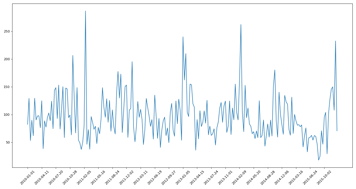
练习1:统计出911数据中不同月份的电话次数
import pandas as pd
from matplotlib import pyplot as plt

file_path = './911.csv'
df = pd.read_csv(file_path)
pd.set_option('display.max_rows', 30)
pd.set_option('display.max_columns', 9)

'''

RangeIndex: 249737 entries, 0 to 249736
Data columns (total 9 columns):
 #   Column     Non-Null Count   Dtype
 0   No               52584 non-null  int64
 1   year             52584 non-null  int64
 2   month            52584 non-null  int64
 3   day              52584 non-null  int64
 4   hour             52584 non-null  int64
 5   season           52584 non-null  int64
 6   PM_Dongsi        25052 non-null  float64
 7   PM_Dongsihuan    20508 non-null  float64
 8   PM_Nongzhanguan  24931 non-null  float64
 9   PM_US Post       50387 non-null  float64
 10  DEWP             52579 non-null  float64
 11  HUMI             52245 non-null  float64
 12  PRES             52245 non-null  float64
 13  TEMP             52579 non-null  float64
 14  cbwd             52579 non-null  object
 15  Iws              52579 non-null  float64
 16  precipitation    52100 non-null  float64
 17  Iprec            52100 non-null  float64
dtypes: float64(11), int64(6), object(1)
memory usage: 7.2+ MB
None'''
pd.set_option('display.max_rows', 30)
pd.set_option('display.max_columns', 18)

'''
   No  year  month  day  hour  season  PM_Dongsi  PM_Dongsihuan  \
0   1  2010      1    1     0       4        NaN            NaN
1   2  2010      1    1     1       4        NaN            NaN
2   3  2010      1    1     2       4        NaN            NaN
3   4  2010      1    1     3       4        NaN            NaN
4   5  2010      1    1     4       4        NaN            NaN

   PM_Nongzhanguan  PM_US Post  DEWP  HUMI    PRES  TEMP cbwd    Iws  \
0              NaN         NaN -21.0  43.0  1021.0 -11.0   NW   1.79
1              NaN         NaN -21.0  47.0  1020.0 -12.0   NW   4.92
2              NaN         NaN -21.0  43.0  1019.0 -11.0   NW   6.71
3              NaN         NaN -21.0  55.0  1019.0 -14.0   NW   9.84
4              NaN         NaN -20.0  51.0  1018.0 -12.0   NW  12.97

   precipitation  Iprec
0            0.0    0.0
1            0.0    0.0
2            0.0    0.0
3            0.0    0.0
4            0.0    0.0
'''

periods = pd.PeriodIndex(year=df["year"], month=df["month"], day=df["day"], hour=df["hour"], freq="H")

'''
PeriodIndex(['2010-01-01 00:00', '2010-01-01 01:00', '2010-01-01 02:00',
             '2010-01-01 03:00', '2010-01-01 04:00', '2010-01-01 05:00',
             '2010-01-01 06:00', '2010-01-01 07:00', '2010-01-01 08:00',
             '2010-01-01 09:00',
             ...

             '2015-12-31 14:00', '2015-12-31 15:00', '2015-12-31 16:00',
             '2015-12-31 17:00', '2015-12-31 18:00', '2015-12-31 19:00',
             '2015-12-31 20:00', '2015-12-31 21:00', '2015-12-31 22:00',
             '2015-12-31 23:00'],
            dtype='period[H]', length=52584, freq='H')
'''
df['datetime'] = periods
df.set_index('datetime',inplace=True)

'''
                  No  year  month  day  hour  season  PM_Dongsi  \
datetime
2010-01-01 00:00   1  2010      1    1     0       4        NaN
2010-01-01 01:00   2  2010      1    1     1       4        NaN
2010-01-01 02:00   3  2010      1    1     2       4        NaN
2010-01-01 03:00   4  2010      1    1     3       4        NaN
2010-01-01 04:00   5  2010      1    1     4       4        NaN

                  PM_Dongsihuan  PM_Nongzhanguan  PM_US Post  DEWP  HUMI  \
datetime
2010-01-01 00:00            NaN              NaN         NaN -21.0  43.0
2010-01-01 01:00            NaN              NaN         NaN -21.0  47.0
2010-01-01 02:00            NaN              NaN         NaN -21.0  43.0
2010-01-01 03:00            NaN              NaN         NaN -21.0  55.0
2010-01-01 04:00            NaN              NaN         NaN -20.0  51.0

                    PRES  TEMP cbwd    Iws  precipitation  Iprec
datetime
2010-01-01 00:00  1021.0 -11.0   NW   1.79            0.0    0.0
2010-01-01 01:00  1020.0 -12.0   NW   4.92            0.0    0.0
2010-01-01 02:00  1019.0 -11.0   NW   6.71            0.0    0.0
2010-01-01 03:00  1019.0 -14.0   NW   9.84            0.0    0.0
2010-01-01 04:00  1018.0 -12.0   NW  12.97            0.0    0.0
'''

df = df.resample('10D').mean()

data = df['PM_US Post'].dropna()

'''
datetime
2010-01-01 23:00    129.0
2010-01-02 00:00    148.0
2010-01-02 01:00    159.0
2010-01-02 02:00    181.0
2010-01-02 03:00    138.0
                    ...

2015-12-31 19:00    133.0
2015-12-31 20:00    169.0
2015-12-31 21:00    203.0
2015-12-31 22:00    212.0
2015-12-31 23:00    235.0
Freq: H, Name: PM_US Post, Length: 50387, dtype: float64
'''
x = data.index
y = data.values
plt.figure(figsize=(15,8),dpi=80)
plt.plot(range(len(x)),y)
plt.xticks(range(0,len(x),10),list(x)[::10],rotation=45)
plt.show()
四、pandas画图
1.折线图
from matplotlib import pyplot as plt
import pandas as pd
iris_data = pd.read_csv(‘iris.csv’)
”’
RangeIndex: 150 entries, 0 to 149
Data columns (total 5 columns):
# Column Non-Null Count Dtype
Original: https://blog.csdn.net/yangyusir/article/details/115145492
Author: yangyusir
Title: 数据分析 第七讲 pandas练习 数据的合并、分组聚合、时间序列、pandas绘图
原创文章受到原创版权保护。转载请注明出处:https://www.johngo689.com/767448/
转载文章受原作者版权保护。转载请注明原作者出处!