【Python】数字图像分析

图像处理

• 一、环境配置
• 二、图像分析
  *
• [1] skimage.io.imread(fname,as_gray)
• [2] skimage.io.imshow(img,cmap)
• [3] skimage.io.show()
• [4] matplotlib.pyplot.figure(num=None, figsize=None, dpi=None, facecolor=None, edgecolor=None, frameon=True, clear=False)
• [5] matplotlib.pyplot.subplot(nrows, ncols, plot_number)
• [6] matplotlib.pyplot.axis([xmin, xmax, ymin, ymax],option)
• [7] matplotlib.pyplot.subplots(nrows, ncols,num, figsize, dpi, facecolor, edgecolor)
• [8] matplotlib.pyplot.tight_layout(pad, h_pad, w_pad, rect)
• [9] skimage.img_as_float & skimage.img_as_ubyt & skimage.img_as_uint & skimage.img_as_int
• [10] skimage.color.rgb2gray(rgb) & skimage.color.rgb2hsv(rgb) & skimage.color.rgb2lab(rgb) & skimage.color.gray2rgb(image) & skimage.color.hsv2rgb(hsv) & skimage.color.lab2rgb(lab)
• [11] skimage.color.convert_colorspace(arr, fromspace, tospace)
• [12] skimage.color.label2rgb(arr)
• [13] skimage.io.ImageCollection(load_pattern,load_func)
• [14] skimage.io.concatenate_images(ic)
• [15] skimage.transform.resize(image,output_shape)
• [16] skimage.transform.rescale(image, scale[, …])
• [17] skimage.transform.rotate(image, angle[, …],resize=False)
• [18] skimage.transform.pyramid_gaussian(image, downscale=2)
• [19] skimage.exposure.adjust_gamma(image, gamma) & skimage.exposure.adjust_log(image, gain)
• [20] skimage.exposure.is_low_contrast(img)
• [21] skimage.exposure.rescale_intensity(image, in_range, out_range)
• [22] skimage.exposure.histogram(image, nbins)
• [23] matplotlib.pyplot.hist(arr, bins=10, normed=0, facecolor=’black’, edgecolor=’black’,alpha=1，histtype=’bar’)
• [24] skimage.exposure.equalize_hist(image, nbins=256, mask=None)
• [25] skimage.filters.sobel(image, mask=None) & skimage.filters.roberts(image, mask=None) & skimage.filters.scharr(image, mask=None) & skimage.filters.prewitt(image, mask=None) & skimage.feature.canny(image, sigma=1.0)
• [26] skimage.filters.roberts_neg_diag(image) & skimage.filters.roberts_pos_diag(image)
• [27] skimage.filters.gaussian(image, sigma)
• [28] skimage.filters.median(image)
• [29] skimage.filters.threshold_otsu(image, nbins=256) & skimage.filters.threshold_yen(image) & skimage.filters.threshold_li(image) & skimage.filters.threshold_isodata(image)
• [30] skimage.filters.threshold_local(image, block_size, method=’gaussian’）
• [31] skimage.draw.line(r1,c1,r2,c2)
• [32] skimage.draw.circle(cy, cx, radius) & skimage.draw.circle_perimeter(yx,yc,radius)
• [33] skimage.draw.bezier_curve(y1,x1,y2,x2,y3,x3,weight)
• [34] skimage.draw.ellipse_perimeter(cy, cx, yradius, xradius）
• [35] skimage.draw.polygon(Y,X)

一、环境配置

scipy是科学和工程领域的软件包

pip install scipy

numpy用于存储和处理大型矩阵

pip install numpy

scikit-image，图片处理工具

pip install scikit-image

2D绘图的数据可视化工具matplotlib

pip install matplotlib

二、图像分析

skimage模块下有许多子模块，用到一些模块中的操作函数就需要导入对应的模块，导入多个模块要用逗号分隔。

子模块功能io读取、保存和显示图片或视频data提供一些测试图片和样本数据color颜色空间变换filters图片增强、边缘检测、排序滤波器、自动阈值等等draw操作用于numpy数组上的基本图形绘制，包括线条、矩形、园和文本等transform几何变换或者其它变换，如旋转、拉伸和拉东变换等morphology形态学操作，如开闭运算、股价提取等等exposure图片强度调整，如亮度调整、直方图均衡等feature特征检测与提取等measure图像属性的测量，如相似性或者等高线等segmentation图像分割restoration图像恢复util通用函数

[1] skimage.io.imread(fname,as_gray)

实现对图片的简单获取，返回一个 numpy的 ndarray数组

• fname：图片的路径
• as_gray：布尔值，表示是否读取灰度照片，默认False

通过这个numpy数组可以访问图片的像素点

img[i,j,c]

灰度图片访问方式

gray[i,j]

配合数组切片，还可以进行图片截取，通道提取等等

img_R=img[:,:,0]
img_G=img[:,:,1]
img_B=img[:,:,2]

img_1=img[40:140,100:200,:]

img[i,:] = img[j,:]

img[:,i] = 100

img[:100,:50].sum()

img[i].mean()

img[:,-1]

img[-2,:]

[2] skimage.io.imshow(img,cmap)

对 一个图片或者 numpy数组进行图像绘制，实质是用 matplotlib对图片绘制，返回一个 matplotlib数据。

from skimage import io,data
io.imshow(r"E:\Image\PictureForWindows\load_wallpaper_list\530895_souredapple_clouds.png")
io.show()

既然是用的 matplotlib，那么也可等价于

import matplotlib.pyplot as plt
plt.imshow(img)

参数有如下含义：

• img:要绘制的图像的 路径字符串或者 numpy数组
• cmap：选择颜色图谱，默认绘制 RGB(A)颜色空间

颜色图谱描述autumn红-橙-黄bone黑-白，x线cool青-洋红copper黑-铜flag红-白-蓝-黑gray黑-白hot黑-红-黄-白hsvhsv颜色空间， 红-黄-绿-青-蓝-洋红-红inferno黑-红-黄jet蓝-青-黄-红magma黑-红-白pink黑-粉-白plasma绿-红-黄prism红-黄-绿-蓝-紫-…-绿模式spring洋红-黄summer绿-黄viridis蓝-绿-黄winter蓝-绿

[3] skimage.io.show()

打开查看器，要想把绘制的图片在窗口显示，就需要用这个函数

from skimage import io
import matplotlib.pyplot as plt

img_1=io.imread(r"E:\Image\530895_souredapple_clouds.png")

img_2=io.imread(r"E:\Image\530895_souredapple_clouds.png",as_gray=True)

io.imshow(img_1,plt.cm.winter)

io.show()

io.imshow(img_2,cmap=plt.cm.autumn)

io.show()

在上面的实现代码中，两张图片显示两次，要想让几张图片显示在一个窗口中可以搭配使用figure函数和subplot函数

[4] matplotlib.pyplot.figure(num=None, figsize=None, dpi=None, facecolor=None, edgecolor=None, frameon=True, clear=False)

设置绘图窗口大小等。

• num:这个参数是一个可选参数，即可以给参数也可以不给参数。可以将该num理解为窗口的属性id,即该窗口的身份标识。如果不提供该参数，则创建窗口的时候该参数会自增，如果提供的话则该窗口会以该num为Id存在。
• figsize:可选参数。整数元组，默认是无。提供整数元组则会以该元组为长宽。例如（4，4）即以长4英寸 宽4英寸的大小创建一个窗口
• dpi：可选参数，整数。表示该窗口的分辨率，如果没有提供则默认为 figure.dpi
• facecolor：可选参数，表示窗口的背景颜色，如果没有提供则默认为figure.facecolor，其中颜色的设置是通过RGB，范围是’#000000’~’#FFFFFF’，其中每2个字节16位表示RGB的0-255，例如’#FF0000’表示R:255 G:0 B:0 即红色。
• edgecolor:可选参数，表示窗口的边框颜色，如果没有提供则默认为figure,edgecolor
• frameon:可选参数，表示是否绘制窗口的图框，默认是
• figureclass：暂不了解
• clear:可选参数，默认是false,如果提供参数为ture，并且该窗口存在的话 则该窗口内容会被清除。

[5] matplotlib.pyplot.subplot(nrows, ncols, plot_number)

划分子图

• nrows:子图的行数
• ncols:子图的列数
• plot_number当前子图编号

[6] matplotlib.pyplot.axis([xmin, xmax, ymin, ymax],option)

设置坐标轴，

• [xmin, xmax, ymin, ymax]:设置坐标轴的范围
• option:可以是bool值或者字符串， 'off'相当于 False（隐藏坐标轴）， 'on'相当于 True

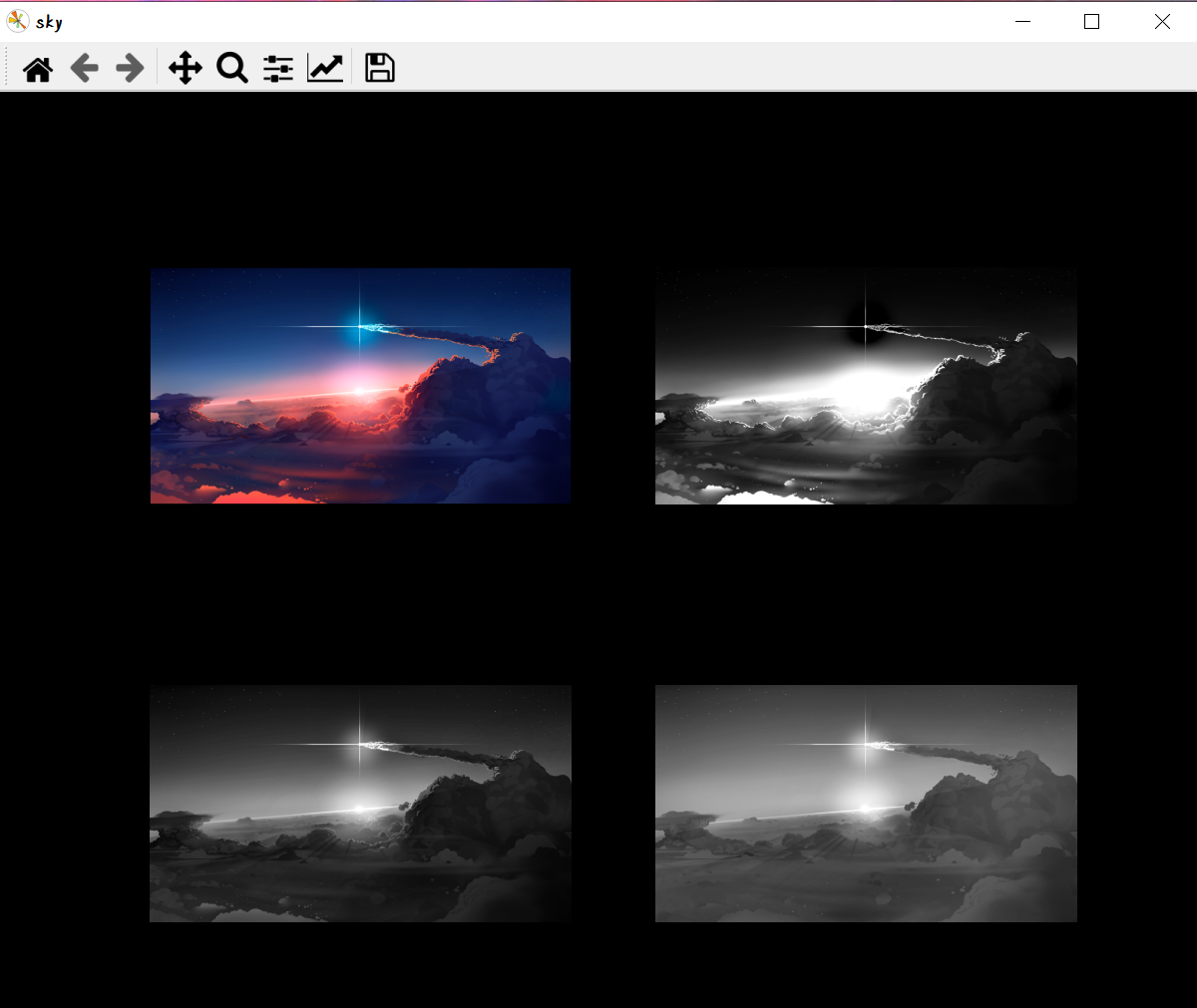
from skimage import io
import matplotlib.pyplot as plt
img=io.imread(r"E:\Image\530895_souredapple_clouds.png")

plt.figure(num='sky',figsize=(8,8),facecolor='black')

plt.subplot(2,2,1)
plt.title('original image')
plt.imshow(img)

plt.subplot(2,2,2)
plt.title('Channel R')
plt.imshow(img[:,:,0],cmap=plt.cm.gray)
plt.axis('off')

plt.subplot(2,2,3)
plt.title('Channel G')
plt.imshow(img[:,:,1],cmap=plt.cm.gray)
plt.axis('off')

plt.subplot(2,2,4)
plt.title('Channel B')
plt.imshow(img[:,:,2],cmap=plt.cm.gray)
plt.axis('off')

plt.show()

效果如下：

[7] matplotlib.pyplot.subplots(nrows, ncols,num, figsize, dpi, facecolor, edgecolor)

创建多子图的窗口，返回一个窗口和一个 tuple型的对象，每个元素代表一个子图

• nrows:所有子图的行数，默认为1
• ncols:所有子图的列数，默认为1
• 其他的参数跟figure函数的一样，不再赘述

[8] matplotlib.pyplot.tight_layout(pad, h_pad, w_pad, rect)

用于多个子图情况下调整显示的布局

• pad:主窗口边缘和子图边缘的间距，默认 1.08
• h_pad, w_pad: 子图边缘之间的间距，默认为 pad_inches
• rect: 一个矩形区域，如果设置这个值，则将所有的子图调整到这个矩形区域内。

from skimage import io
import matplotlib.pyplot as plt
img=io.imread(r"E:\Image\530895_souredapple_clouds.png")

window,ax=plt.subplots(2,2,figsize=(8,8),facecolor='black')

plt.tight_layout(4)

ax0,ax1,ax2,ax3=ax.ravel()

ax0.set_title("Original Image")
ax1.set_title("Channel R")
ax2.set_title("Channel G")
ax3.set_title("Channel B")

ax0.imshow(img)
ax1.imshow(img[:,:,0],cmap=plt.cm.gray)
ax2.imshow(img[:,:,1],cmap=plt.cm.gray)
ax3.imshow(img[:,:,2],cmap=plt.cm.gray)

plt.show()

先简单总结一下一些绘图用到的函数

函数名功能调用格式figure创建一个显示窗口plt.figure(num=1,figsize=(8,8)imshow绘制图片plt.imshow(image)show显示窗口plt.show()subplot划分子图plt.subplot(2,2,1)title设置子图标题(与subplot结合使用）plt.title(‘origin image’)axis是否显示坐标尺plt.axis(‘off’)subplots创建带有多个子图的窗口fig,axes=plt.subplots(2,2,figsize=(8,8))ravel为每个子图设置变量ax0,ax1,ax2,ax3=axes.ravel()set_title设置子图标题（与axes结合使用）ax0.set_title(‘first window’)tight_layout自动调整子图显示布局plt.tight_layout()

[9] skimage.img_as_float & skimage.img_as_ubyt & skimage.img_as_uint & skimage.img_as_int

一张图片其实是以numpy的ndarray数组的形式存储的，对这个数组如何进行数据类型的转换，可以用下面的函数，但在调用之前需要import导入

from skimage import img_as_float,img_as_ubyte,img_as_uint,img_as_int

Function nameDescriptionimg_as_floatConvert to 64-bit floating point.img_as_ubyteConvert to 8-bit uint.img_as_uintConvert to 16-bit uint.img_as_intConvert to 16-bit int.

一张彩色图片转换为灰度图后，它的类型就由 unit8变成了 float，
可以通过img_as_float()函数将unit8类型转换为float型，实际上还有更简单的方法，就是乘以1.0

[10] skimage.color.rgb2gray(rgb) & skimage.color.rgb2hsv(rgb) & skimage.color.rgb2lab(rgb) & skimage.color.gray2rgb(image) & skimage.color.hsv2rgb(hsv) & skimage.color.lab2rgb(lab)

实现rgb、hsv、cmyk、gray（灰度空间）这几个颜色空间之间的转换

[11] skimage.color.convert_colorspace(arr, fromspace, tospace)

是 [9]的整合，将arr从fromspace颜色空间转换到tospace颜色空间。

[12] skimage.color.label2rgb(arr)

用arr数组给图片着色

from skimage import io,data,color
import numpy as np
img=io.imread(r"E:\Image\530895_souredapple_clouds.png")

img_gray=color.rgb2gray(img)
'''print(gray[0,0])'''

row,col=img_gray.shape

label=np.zeros([row,col])
'''print(label)'''

for i in range(row):
    for j in range(col):
        if img_gray[i,j]<0.4:
            label[i,j]=1
        elif img_gray[i,j]<0.75:
            label[i,j]=2
        else:
            label[i,j]=3
'''print(label)'''

img_label=color.label2rgb(label)
io.imshow(img_label)
io.show()

[13] skimage.io.ImageCollection(load_pattern,load_func)

对 load_pattern路径的图片组批量用 load_func函数处理（默认是 imread），返回各个图片路径作为元素组成的列表。

[14] skimage.io.concatenate_images(ic)

将图片连接起来，构成一个维度更高的数组， ic是目标图片路径字符串的列表（图片的集合），但这些图片的大小必须要一致。

'''
将Image文件夹下的图片设置同一大小之后存入test文件夹下，然后连接
'''
from skimage import io,data,color,transform
import numpy as np
import os

try:
    path='E:\\test'
    if not os.path.exists(path):
        os.makedirs(path)
        print("创建目录成功")
except BaseException as msg:
    print("新建目录失败：" + msg)

def convert_gray(f):
    rgb = io.imread(f)
    return color.rgb2gray(rgb)

def resize_(f):
    img=io.imread(f)
    img=transform.resize(img,(100,100))
    return img

coll_1=io.ImageCollection(r"E:\Image\*.png",load_func=resize_)

for i in range(len(coll_1)):
    io.imsave(r"E:/test/{}.png".format(i),coll_1[i])

coll_2=io.ImageCollection(r"E:\test\*.png")
io.imshow(coll_2[0])
io.show()

coll_3=io.concatenate_images(coll_2)

print(coll_3.shape)

skimage的 transform子模块用于图像的形变与缩放

[15] skimage.transform.resize(image,output_shape)

给目标图片设置新的大小，函数返回调整后的图片（ndarray数组）

• image:代表目标图片的ndarray数组
• output_shape:新的图片尺寸，可以是元组也可以是ndarray数组

[16] skimage.transform.rescale(image, scale[, …])

给目标图片按照scale缩放，函数返回调整后的图片（ndarray数组）

• image:代表目标图片的ndarray数组
• scale:scale参数可以是 单个float数，表示缩放的倍数；也可以是一个 float型的列表，如[0.2,0.5],表示将行列数分开进行缩放

[17] skimage.transform.rotate(image, angle[, …],resize=False)

使目标图片旋转angle度数，函数返回调整后的图片（ndarray数组）

• angle:参数是个float类型数，表示旋转的度数
• resize:用于控制在旋转时，是否改变大小 ，默认为False

[18] skimage.transform.pyramid_gaussian(image, downscale=2)

图像金字塔是以多分辨率来解释图像的一种有效但概念简单的结构。图像金字塔最初用于机器视觉和图像压缩，一幅图像的金字塔是一系列以金字塔形状排列的分辨率逐步降低的图像集合。金字塔的底部是待处理图像的高分辨率表示，而顶部是低分辨率的近似。当向金字塔的上层移动时，尺寸和分辨率就降低。

生成一个高斯金字塔。

• downscale:代表缩放比例
• 其他的参数含义在导入相关库之后可以用python内置的help函数获取 print(help(transform.pyramid_gaussian))

'''
如何根据图片生成一个高斯金字塔并显示出来
'''
import numpy as np
import matplotlib.pyplot as plt
from skimage import data,transform

image = data.astronaut()

rows, cols, dim = image.shape

'''
#查看transform.pyramid_gaussian具体用法
print(help(transform.pyramid_gaussian))
'''

pyramid = tuple(transform.pyramid_gaussian(image, downscale=2, multichannel=True))

'''
#分别查看金字塔的各个图像
plt.imshow(pyramid[0])
plt.show()
plt.imshow(pyramid[1])
plt.show()
plt.imshow(pyramid[2])
plt.show()
'''

complex_image = np.ones((rows, int(cols + cols / 2), 3), dtype=np.double)

complex_image[:rows, :cols, :dim] = pyramid[0]

i_row = 0
for p in pyramid[1:]:
    n_rows, n_cols = p.shape[:2]

    complex_image[i_row:i_row + n_rows, cols:cols + n_cols,:] = p
    i_row += n_rows

plt.imshow(complex_image)
plt.show()

图像亮度与对比度的调整还有直方图的处理，是放在 skimage包的 exposure模块里面

[19] skimage.exposure.adjust_gamma(image, gamma) & skimage.exposure.adjust_log(image, gain)

adjust_gamma原理：I = I g I = I^g I =I g
对原图像的像素进行幂运算，得到新的像素值。公式中的g就是gamma值。

• 如果 gamma>1, 新图像比原图像 暗。
• 如果 gamma<1< code>,&#x65B0;&#x56FE;&#x50CF;&#x6BD4;&#x539F;&#x56FE;&#x50CF;<code>&#x4EAE;</code>&#x3002;<!--1<-->

adjust_log原理：与adjust_gamma相反。

设置图片亮度，其中 gamma参数默认为1， gain参数默认为1，返回调整后的 ndarray数组

from skimage import data, exposure, img_as_float
import matplotlib.pyplot as plt
image = img_as_float(data.moon())

gam1= exposure.adjust_gamma(image, 2)
gam2= exposure.adjust_log(image, 2)

plt.figure(num='moon',figsize=(8,8),facecolor='white')

plt.subplot(1,3,1)
plt.title("original")
plt.imshow(image)

plt.subplot(1,3,2)
plt.title("dark")
plt.imshow(gam1)

plt.subplot(1,3,3)
plt.title("bright")
plt.imshow(gam2)

plt.show()

[20] skimage.exposure.is_low_contrast(img)

判断图像对比度是否偏低，返回一个bool型值

[21] skimage.exposure.rescale_intensity(image, in_range, out_range)

用于调整强度，相当于把处于 in_range范围中image的像素值映射到 out_range范围，得到一个新的像素值。

• in_range:输入图片的强度范围，默认是image的最大像素值和最小像素值
• out_range:输出图片的强度范围，默认是图像类型的最大值和最小值，例如如果dtype=uint8，那么out_range=[0,255]。

'''
测试该函数的用法与效果
'''
from skimage import exposure
import numpy as np

'''设置了3种类型的image'''
image1 = np.array([51, 102, 153], dtype=np.uint8)
image2 = image1*1.0
image3 = np.array([-10, 0, 10], dtype=np.int8)

'''uint8型image的默认输入'''
mat=exposure.rescale_intensity(image1)
print(mat)

'''image转小数之后，下面两个等价，对image进行了拉伸'''
mat=exposure.rescale_intensity(image2,in_range=(51,153),out_range=(0,1))
print(mat)
mat=exposure.rescale_intensity(image2)
print(mat)

'''等比例缩小，相当于原像素除以255'''
mat=exposure.rescale_intensity(image2,in_range=(0,255))
print(mat)
mat=exposure.rescale_intensity(image2,in_range=(0,255),out_range=(0,1))
print(mat)

'''等比例缩小，但image超出了(0,102)的范围，相当于原像素除以102，超出1的变1'''
mat=exposure.rescale_intensity(image2,in_range=(0,102))
print(mat)

'''负数调整为正数'''
mat=exposure.rescale_intensity(image3, out_range=(0, 127))
print(mat)

直方图：确定图像像元的灰度值范围，以适当的灰度间隔为单位将其划分为若干等级，横轴是灰度级，纵轴是像元数或该像元数占总像元数的比例值，做出的条形统计图即为灰度直方图。
直方图反映了图像中的灰度分布规律，描述不同灰度级具有的像元个数，但不包含这些像元在图像中所处的位置。
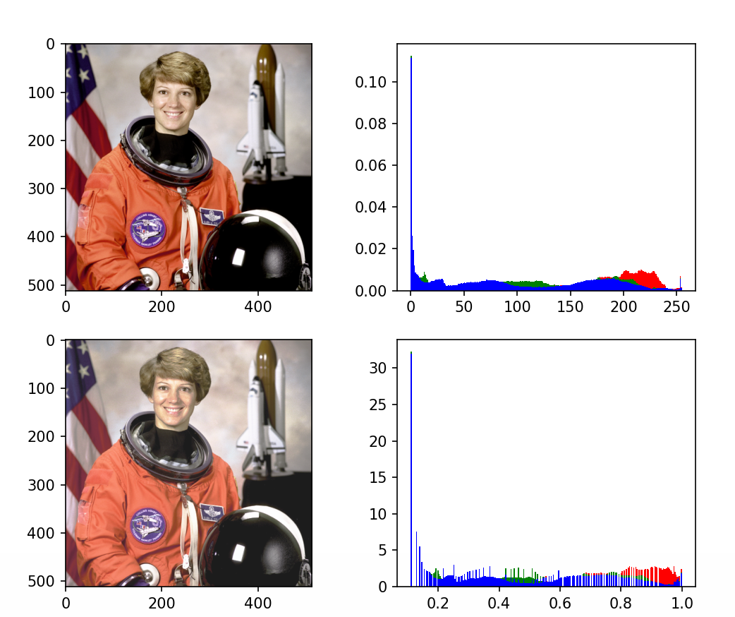
直方图均衡化：如果一副图像的像素占有很多的灰度级而且分布均匀，那么这样的图像往往有高对比度和多变的灰度色调。直方图均衡化就是一种能仅靠输入图像直方图信息自动达到这种效果的变换函数。它的基本思想是对图像中像素个数多的灰度级进行展宽，而对图像中像素个数少的灰度进行压缩，从而扩展取值的动态范围，提高了对比度和灰度色调的变化，使图像更加清晰。

[22] skimage.exposure.histogram(image, nbins)

用于计算一个图片的直方图。
返回一个tuple，这个tuple有两个数组，前一个是直方图的统计量，后一个是每个柱的中间值，若是用numpy的内置histogram函数就不是中间值，而是每个柱的范围值。

• nbins:柱数，默认是256

import numpy as np
from skimage import exposure,data
image =data.camera()*1.0
hist1=np.histogram(image, bins=4)
hist2=exposure.histogram(image, nbins=4)
print(hist1)
print(hist2)

输出

(array([77570, 16015, 89783, 78776], dtype=int64), array([  0.  ,  63.75, 127.5 , 191.25, 255.  ]))
(array([77570, 16015, 89783, 78776], dtype=int64), array([ 31.875,  95.625, 159.375, 223.125]))

[23] matplotlib.pyplot.hist(arr, bins=10, normed=0, facecolor=’black’, edgecolor=’black’,alpha=1，histtype=’bar’)

实现对直方图的绘制。

• x: 需要计算的直方图的 一维数组，经常要用到numpy包中的flatten()函数，用于将二维数组序列化成一维数组。
• bins: 直方图的柱数，即要分的组数，默认为10；
• range：元组(tuple)或None；剔除较大和较小的离群值，给出全局范围；如果为None，则默认为(x.min(), x.max())；即x轴的范围；
• density：布尔值。如果为true，则返回的元组的第一个参数n将为频率而非默认的频数；
• weights：与x形状相同的权重数组；将x中的每个元素乘以对应权重值再计数；如果density取值为True，则会对权重进行归一化处理。这个参数可用于绘制已合并的数据的直方图；
• cumulative：布尔值；如果为True，则计算累计频数；如果density取值为True，则计算累计频率；
• bottom：数组，标量值或None；每个柱子底部相对于y=0的位置。如果是标量值，则每个柱子相对于y=0向上/向下的偏移量相同。如果是数组，则根据数组元素取值移动对应的柱子；即直方图上下便宜距离；
• histtype： {'bar', 'barstacked', 'step', 'stepfilled'}； 'bar’是传统的条形直方图； 'barstacked’是堆叠的条形直方图； 'step'是未填充的条形直方图，只有外边框； 'stepfilled'是有填充的直方图；当 histtype取值为 'step'或 'stepfilled'， rwidth设置失效，即不能指定柱子之间的间隔，默认连接在一起；
• align： {'left', 'mid', 'right'}； 'left'：柱子的中心位于bins的左边缘； 'mid'：柱子位于bins左右边缘之间； 'right'：柱子的中心位于bins的右边缘；
• orientation： {'horizontal', 'vertical'}：如果取值为horizontal，则条形图将以y轴为基线，水平排列；简单理解为类似bar()转换成barh()，旋转90°；
• rwidth：标量值或None。柱子的宽度占bins宽的比例；
• log：布尔值。如果取值为True，则坐标轴的刻度为对数刻度；如果log为True且x是一维数组，则计数为0的取值将被剔除，仅返回非空的(frequency, bins, patches）；
• color：具体颜色，数组（元素为颜色）或None。
• label：字符串（序列）或None；有多个数据集时，用label参数做标注区分；
• stacked：布尔值。如果取值为True，则输出的图为多个数据集堆叠累计的结果；如果取值为False且 histtype='bar'或 'step'，则多个数据集的柱子并排排列；

返回值如下：

• n: 直方图向量，是否归一化由参数normed设定
• bins: 返回各个bin的区间范围
• patches: 返回每个bin里面包含的数据，是一个list

[24] skimage.exposure.equalize_hist(image, nbins=256, mask=None)

直方图均衡化，返回均衡化之后的图像。

• image：图像数组
• nbins：图像直方图的桶数。注意：对于整数图像，这个参数被忽略，每个整数都是它自己的桶。
• mask：与图像相同形状的数组。仅使用掩码 == 为真的点进行均衡，将其应用于整个图像。

'''对astronaut图片绘制直方图并均衡化'''
from skimage import io,data,exposure
import matplotlib.pyplot as plt
import numpy as np
img = data.astronaut()

plt.figure("hist",figsize=(8,8))

plt.subplot(2,2,1)
plt.imshow(img)

plt.subplot(2,2,2)
ar=img[:,:,0].flatten()
plt.hist(ar, bins=256, color='r',density=1,histtype='bar')
ag=img[:,:,1].flatten()
plt.hist(ag, bins=256, color='g',density=1,histtype='bar')
ab=img[:,:,2].flatten()
plt.hist(ab, bins=256, color='b',density=1,histtype='bar')

plt.subplot(2,2,3)
img1=exposure.equalize_hist(img)
plt.imshow(img1)

plt.subplot(2,2,4)
ar=img1[:,:,0].flatten()
plt.hist(ar, bins=256, color='r',density=1,histtype='bar')
ag=img1[:,:,1].flatten()
plt.hist(ag, bins=256, color='g',density=1,histtype='bar')
ab=img1[:,:,2].flatten()
plt.hist(ab, bins=256, color='b',density=1,histtype='bar')

plt.show()

skimage库中通过 filters模块进行滤波操作和阈值分割。

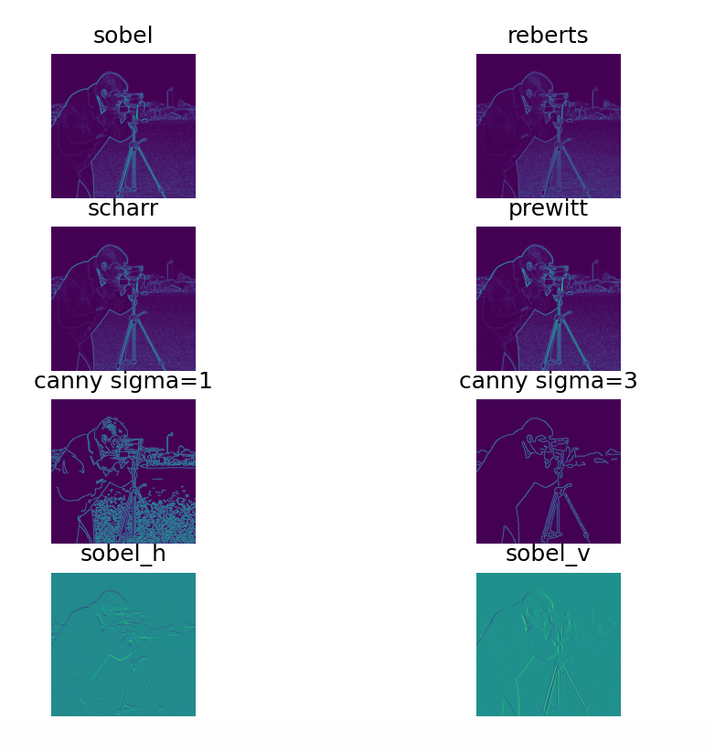
[25] skimage.filters.sobel(image, mask=None) & skimage.filters.roberts(image, mask=None) & skimage.filters.scharr(image, mask=None) & skimage.filters.prewitt(image, mask=None) & skimage.feature.canny(image, sigma=1.0)

这些都是用于检测边缘，而对于canny算子，sigma越小，边缘线条越细小。

• 要是想只水平边缘检测可以用 sobel_h, prewitt_h, scharr_h
• 要是想只垂直边缘检测可以用 sobel_v, prewitt_v, scharr_v

'''绘制用不同算子进行边缘检测之后的效果图片'''
from skimage import data,filters,feature
import matplotlib.pyplot as plt
import numpy as np
img = data.camera()
plt.figure("检测边缘",figsize=(8,8))

plt.subplot(4,2,1)
plt.title("sobel")
img1=filters.sobel(img)
plt.imshow(img1)
plt.axis('off')

plt.subplot(4,2,2)
plt.title("reberts")
img2=filters.roberts(img)
plt.imshow(img2)
plt.axis('off')

plt.subplot(4,2,3)
plt.title("scharr")
img3=filters.scharr(img)
plt.imshow(img3)
plt.axis('off')

plt.subplot(4,2,4)
plt.title("prewitt")
img4=filters.prewitt(img)
plt.imshow(img4)
plt.axis('off')

plt.subplot(4,2,5)
plt.title("canny sigma=1")
img5=feature.canny(img)
plt.imshow(img5)
plt.axis('off')

plt.subplot(4,2,6)
plt.title("canny sigma=3")
img6=feature.canny(img,sigma=3)
plt.imshow(img6)
plt.axis('off')

plt.subplot(4,2,7)
plt.title("sobel_h")
img7=filters.sobel_h(img)
plt.imshow(img7)
plt.axis('off')

plt.subplot(4,2,8)
plt.title("sobel_v")
img8=filters.sobel_v(img)
plt.imshow(img8)
plt.axis('off')

plt.show()

效果如下：

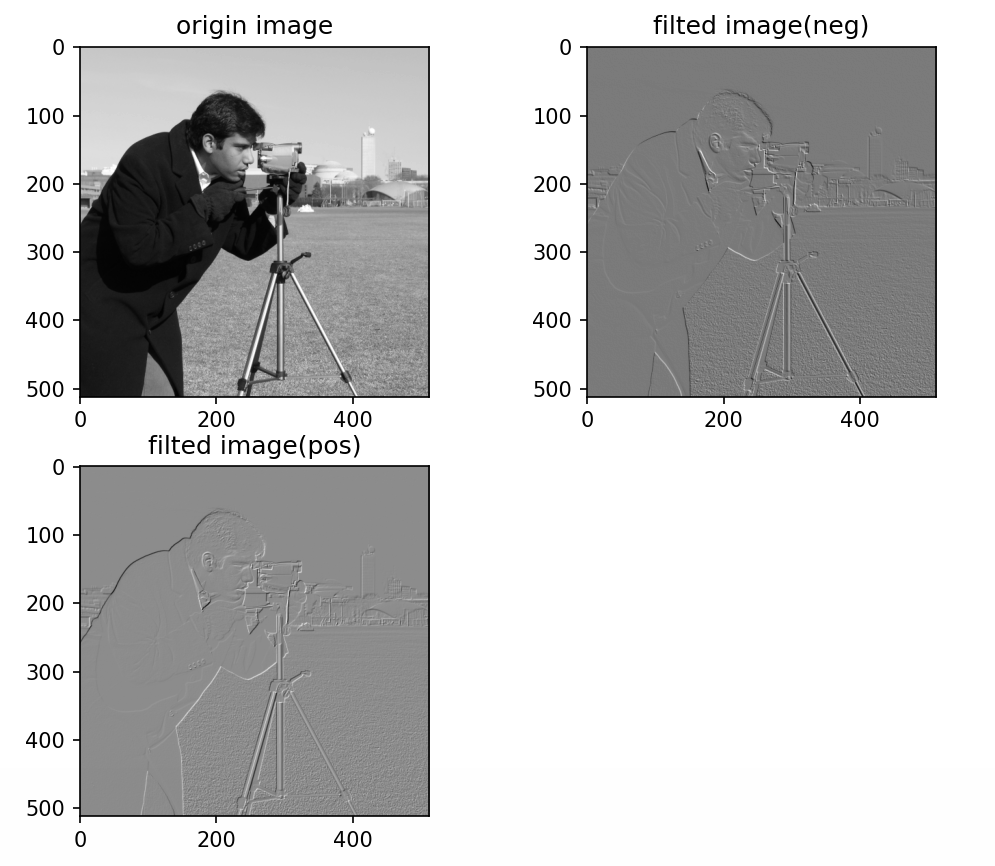
[26] skimage.filters.roberts_neg_diag(image) & skimage.filters.roberts_pos_diag(image)

两个函数都是交叉边缘检测。

from skimage import data,filters
import matplotlib.pyplot as plt
img =data.camera()
dst_1=filters.roberts_neg_diag(img)
dst_2=filters.roberts_pos_diag(img)

plt.figure('filters',figsize=(8,8))

plt.subplot(2,2,1)
plt.title('origin image')
plt.imshow(img,plt.cm.gray)

plt.subplot(2,2,2)
plt.title('filted image')
plt.imshow(dst_1,plt.cm.gray)

plt.subplot(2,2,3)
plt.title('filted image')
plt.imshow(dst_2,plt.cm.gray)

plt.show()

在进行接下来的学习前，先了解两个概念：噪声与高斯噪声。

• 噪声在图像当中常表现为一引起较强视觉效果的孤立像素点或像素块。简单来说，噪声的出现会给图像带来干扰，让图像变得不清楚。
• 高斯噪声就是它的概率密度函数服从高斯分布（即正态分布）的一类噪声。如果一个噪声，它的幅度分布服从高斯分布，而它的功率谱密度又是均匀分布的，则称它为高斯白噪声。高斯白噪声的二阶矩不相关，一阶矩为常数，是指先后信号在时间上的相关性。

[27] skimage.filters.gaussian(image, sigma)

gaussian滤波，通过调节sigma的值来调整滤波效果，可以消除高斯噪声
sigma越大，过滤之后的图像越模糊

[28] skimage.filters.median(image)

中值滤波，一种平滑滤波，可以消除噪声。需要用 skimage.morphology模块来设置滤波器的形状。

from skimage import data,filters
import matplotlib.pyplot as plt
from skimage.morphology import disk
img = data.camera()
edges1 = filters.median(img,disk(5))
edges2= filters.median(img,disk(9))
edges3 = filters.gaussian(img,sigma=0.4)
edges4 = filters.gaussian(img,sigma=5)

plt.figure('median',figsize=(8,8))

plt.subplot(2,2,1)
plt.title("median disk(5)")
plt.imshow(edges1,plt.cm.gray)
plt.axis('off')

plt.subplot(2,2,2)
plt.title("median disk(9)")
plt.imshow(edges2,plt.cm.gray)
plt.axis('off')

plt.subplot(2,2,3)
plt.title("gaussian sigma=0.4")
plt.imshow(edges3,plt.cm.gray)
plt.axis('off')

plt.subplot(2,2,4)
plt.title("gaussian sigma=5")
plt.imshow(edges4,plt.cm.gray)
plt.axis('off')

plt.show()

图像阈值分割是一种广泛应用的分割技术，利用图像中要提取的目标区域与其背景在灰度特性上的差异，把图像看作具有不同灰度级的两类区域(目标区域和背景区域)的组合，选取一个比较合理的阈值，以确定图像中每个像素点应该属于目标区域还是背景区域，从而产生相应的二值图像。

[29] skimage.filters.threshold_otsu(image, nbins=256) & skimage.filters.threshold_yen(image) & skimage.filters.threshold_li(image) & skimage.filters.threshold_isodata(image)

这几种方法用来自动生成阈值。
其中threshold_otsu是基于 Otsu，自动生成阈值并返回的阈值分割方法， image参数是灰度图像。

'''分割目标区域和背景区域'''
from skimage import data,filters
import matplotlib.pyplot as plt
image = data.camera()

thresh_1 = filters.threshold_otsu(image)
thresh_2 = filters.threshold_yen(image)
thresh_3 = filters.threshold_li(image)
thresh_4 = filters.threshold_isodata(image)

dst_1 =(image  thresh_1)*1.0
dst_2 =(image  thresh_2)*1.0
dst_3 =(image  thresh_3)*1.0
dst_4 =(image  thresh_4)*1.0

plt.figure('thresh',figsize=(8,8))

plt.subplot(3,2,1)
plt.title('original image')
plt.imshow(image,plt.cm.gray)
plt.axis('off')

plt.subplot(3,2,2)
plt.title('binary image(otsu)')
plt.imshow(dst_1,plt.cm.gray)
plt.axis('off')

plt.subplot(3,2,3)
plt.title('binary image(yen)')
plt.imshow(dst_2,plt.cm.gray)
plt.axis('off')

plt.subplot(3,2,4)
plt.title('binary image(li)')
plt.imshow(dst_3,plt.cm.gray)
plt.axis('off')

plt.subplot(3,2,5)
plt.title('binary image(isodata)')
plt.imshow(dst_4,plt.cm.gray)
plt.axis('off')

plt.show()

[30] skimage.filters.threshold_local(image, block_size, method=’gaussian’）

该函数直接访问一个阈值后的图像，而不是阈值。

• block_size: 块大小，指当前像素的相邻区域大小，一般是奇数（如3，5，7。。。）
• method: 用来确定自适应阈值的方法，有’mean’, ‘generic’, ‘gaussian’ 和 ‘median’。默认为gaussian

在skimage包中，draw模块可以进行简单的图形绘制。

[31] skimage.draw.line(r1,c1,r2,c2)

从 r1,c1到 r2,c2画一条线条

[32] skimage.draw.circle(cy, cx, radius) & skimage.draw.circle_perimeter(yx,yc,radius)

第一个是绘制实心圆
第二个是绘制空心圆

[33] skimage.draw.bezier_curve(y1,x1,y2,x2,y3,x3,weight)

绘制贝塞尔曲线

• y1,x1表示第一个控制点坐标
• y2,x2表示第二个控制点坐标
• y3,x3表示第三个控制点坐标
• weight表示中间控制点的权重，用于控制曲线的弯曲度。

[34] skimage.draw.ellipse_perimeter(cy, cx, yradius, xradius）

画空心椭圆。

• cy,cx表示圆心
• yradius,xradius表示长短轴

[35] skimage.draw.polygon(Y,X)

绘制实心多边形。

• Y为多边形顶点的行集合，X为各顶点的列值集合。

参考：

• python数字图像处理】

Original: https://blog.csdn.net/m0_46296905/article/details/119191235
Author: Em0s_Er1t
Title: 【Python】数字图像分析