【李宏毅机器学习CP9】(task3下)PM2.5预测+numpy实现神经网络logistic回归

学习心得

（1）小批量梯度下降算法中，初始参数的选择很重要，不同的初始参数，其对应损失函数收敛速度也不一样
（2）learning rate 采用递减的方式选取的，根据经验的选择也很重要，在实验中多积累、多总结。
（3）注意第二部分的《用numpy实现一个简单神经网络logistic回归模型》中， numpy、h5py、matplotlib、PIL、scipy等库的使用逐渐要练习起来。逻辑回归是最基础也是最重要的模型：

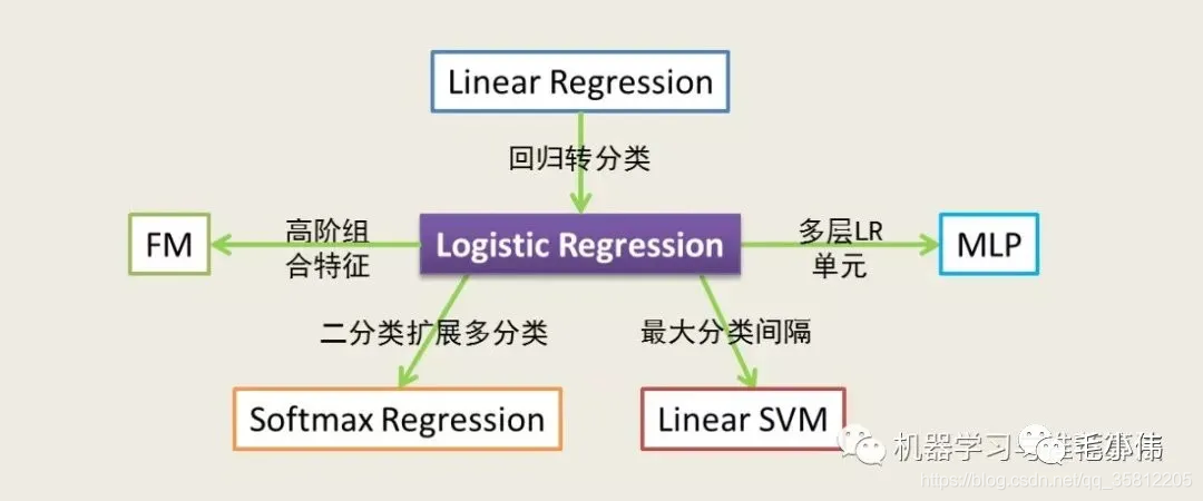
通过逻辑回归能演化出很多模型：

• 逻辑回归=线性回归+sigmoid激活函数，从而将回归问题转换为分类问题
• 逻辑回归+矩阵分解，构成了推荐算法中常用的FM模型
• 逻辑回归+softmax，从而将二分类问题转化为多分类问题
• 逻辑回归还可以看做单层神经网络，相当于最简单的深度学习模型

文章目录

• 学习心得
• 第一部分：PM2.5预测
  *
• 一、作业描述
• 二、任务要求
• 三、大致任务实现
  –
  • 方案1
  • 方案2
  • 方案3
• 第二部分：用numpy实现一个简单神经网络logistic回归模型
  *
• 一、包（库）的介绍
• 二、问题（数据集）概述
  –
  +
  • 练习1：找值
  • 练习2：reshape图片张量
• 三、学习算法的大致框架
• 四、构建自己的算法
  –
  • 1.复习Helper函数
    +
  • 练习3——sigmoid
  • 2.Initializing parameters
    +
  • 练习4——初始化参数为0向量
  • 3.向前传播和向后传播
    +
  • 练习5——传播函数propagate计算损失值和梯度
  • 4.优化器
    +
  • 练习6——优化optimize
  • 练习7——预测predict
• 五、将所有的函数合并成一个模型
  –
  • 练习8——合成model
• 六、拓展分析
• 七、用自己的图片测试
• Reference

; 第一部分：PM2.5预测

一、作业描述

让机器预测到丰原站在下一个小时会观测到的PM2.5。举例来说，现在是2017-09-29 08：00：00 ，那么要预测2017-09-29 09：00：00丰原站的PM2.5值会是多少。

二、任务要求

• 任务要求： 预测PM2.5的值，我们将用 梯度下降法 (Gradient Descent) 预测 PM2.5 的值 (Regression 回归问题)
• 环境要求：
• 要求 python3.5+
• 只能用numpy、scipy、pandas
• 请用梯度下降 手写线性回归
• 最好使用 Public Simple Baseline
• 对于想加载模型而并不想运行整个训练过程的人：
  • 请上传训练代码并命名成 train.py
  • 只要用梯度下降的代码就行了
• 最佳要求：
• 要求 python3.5+
• 任何库都可以用
• 在 Kaggle 上获得你选择的更高的分
• 数据介绍：
  本次作业使用豐原站的觀測記錄，分成 train set 跟 test set，train set 是豐原站每個月的前20天所有資料，test set則是從豐原站剩下的資料中取樣出來。
  train.csv:每個月前20天每個小時的氣象資料(每小時有18種測資)。共12個月。
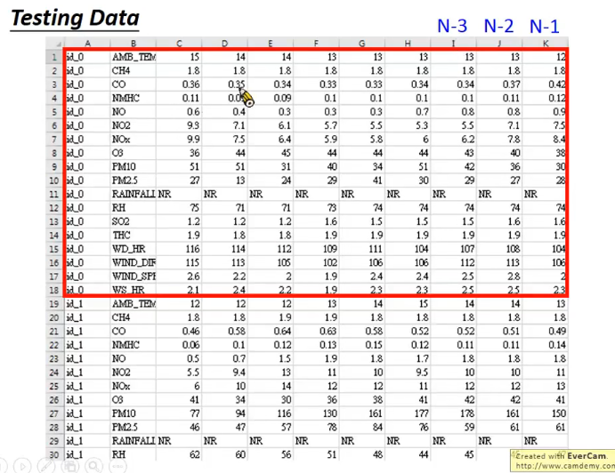
  test.csv:從剩下的資料當中取樣出連續的10小時為一筆，前九小時的所有觀測數據當作feature，第十小時的PM2.5當作answer。一共取出240筆不重複的 test data，請根據feauure預測這240筆的PM2.5。
• 请完成之后参考以下资料：
• Sample_code:https://github.com/datawhalechina/leeml-notes/tree/master/docs/Homework/HW_1

; 三、大致任务实现

步骤：
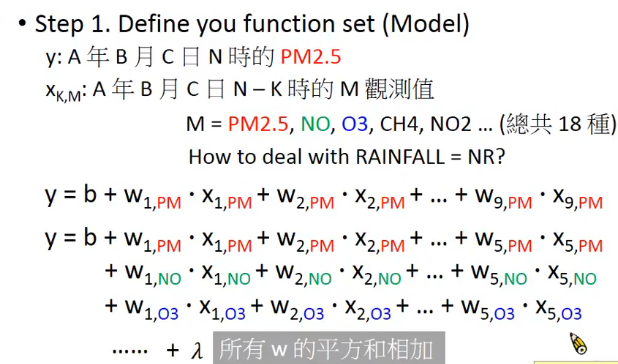
（1）定义你的function set（model），可以加上正则化。

（2）基于training data定义loss function
下图训练资料的每一列为该小时对应的数据。

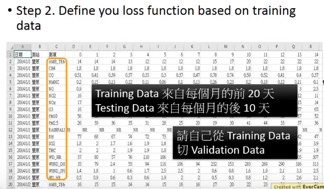
ps：不要将白天的数据当做training data，晚上的数据当做validation data，否则validation data的结果无法反应testing data的结果。

（3）找到最好的function

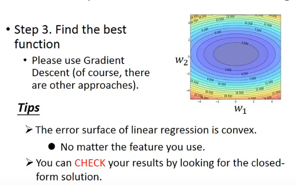
方案1

'''
利用 Linear Regression 线性回归预测 PM2.5
该方法参考黑桃大哥的优秀作业-|vv|-
'''

import numpy as np
import pandas as pd
from sklearn.preprocessing import StandardScaler

path = "./Dataset/"

train = pd.read_csv(path + 'train.csv', engine='python', encoding='utf-8')
test = pd.read_csv(path + 'test.csv', engine='python', encoding='gbk')
train = train[train['observation'] == 'PM2.5']

test = test[test['AMB_TEMP'] == 'PM2.5']

train = train.drop(['Date', 'stations', 'observation'], axis=1)
test_x = test.iloc[:, 2:]

train_x = []
train_y = []

for i in range(15):
    x = train.iloc[:, i:i + 9]

    x.columns = np.array(range(9))
    y = train.iloc[:, i + 9]
    y.columns = np.array(range(1))
    train_x.append(x)
    train_y.append(y)

train_x = pd.concat(train_x)
train_y = pd.concat(train_y)

train_y = np.array(train_y, float)
test_x = np.array(test_x, float)

ss = StandardScaler()

ss.fit(train_x)

train_x = ss.transform(train_x)

ss.fit(test_x)
test_x = ss.transform(test_x)

def r2_score(y_true, y_predict):

    MSE = np.sum((y_true - y_predict) ** 2) / len(y_true)

    return 1 - MSE / np.var(y_true)

class LinearRegression:

    def __init__(self):

        self.coef_ = None
        self.intercept_ = None
        self._theta = None

    def fit_normal(self, X_train, y_train):

        assert X_train.shape[0] == y_train.shape[0], \
            "the size of X_train must be equal to the size of y_train"

        X_b = np.hstack([np.ones((len(X_train), 1)), X_train])
        self._theta = np.linalg.inv(X_b.T.dot(X_b)).dot(X_b.T).dot(y_train)

        self.intercept_ = self._theta[0]
        self.coef_ = self._theta[1:]

        return self

    def fit_gd(self, X_train, y_train, eta=0.01, n_iters=1e4):
        '''
        :param X_train: 训练集
        :param y_train: label
        :param eta: 学习率
        :param n_iters: 迭代次数
        :return: theta 模型参数
        '''

        assert X_train.shape[0] == y_train.shape[0], \
            "the size of X_train must be equal to the size of y_train"

        def J(theta, X_b, y):
            try:
                return np.sum((y - X_b.dot(theta)) ** 2) / len(y)
            except:
                return float('inf')

        def dJ(theta, X_b, y):
            return X_b.T.dot(X_b.dot(theta) - y) * 2. / len(y)

        def gradient_descent(X_b, y, initial_theta, eta, n_iters=1e4, epsilon=1e-8):
            '''
            :param X_b: 输入特征向量
            :param y: lebel
            :param initial_theta: 初始参数
            :param eta: 步长
            :param n_iters: 迭代次数
            :param epsilon: 容忍度
            :return:theta：模型参数
            '''
            theta = initial_theta
            cur_iter = 0

            while cur_iter < n_iters:
                gradient = dJ(theta, X_b, y)
                last_theta = theta
                theta = theta - eta * gradient
                if (abs(J(theta, X_b, y) - J(last_theta, X_b, y)) < epsilon):
                    break
                cur_iter += 1
            return theta

        X_b = np.hstack([np.ones((len(X_train), 1)), X_train])
        initial_theta = np.zeros(X_b.shape[1])
        self._theta = gradient_descent(X_b, y_train, initial_theta, eta, n_iters)
        self.intercept_ = self._theta[0]
        self.coef_ = self._theta[1:]
        return self

    def predict(self, X_predict):

        assert self.intercept_ is not None and self.coef_ is not None, \
            "must fit before predict!"
        assert X_predict.shape[1] == len(self.coef_), \
            "the feature number of X_predict must be equal to X_train"
        X_b = np.hstack([np.ones((len(X_predict), 1)), X_predict])
        return X_b.dot(self._theta)

    def score(self, X_test, y_test):

        y_predict = self.predict(X_test)
        return r2_score(y_test, y_predict)

    def __repr__(self):
        return

LR = LinearRegression().fit_gd(train_x, train_y)

LR.score(train_x, train_y)

result = LR.predict(test_x)

sampleSubmission = pd.read_csv(path + 'sampleSubmission.csv', engine='python', encoding='gbk')
sampleSubmission['value'] = result
sampleSubmission.to_csv(path + 'result.csv')

方案2

import numpy as np
import pandas as pd
import matplotlib.pyplot as plt
import seaborn as sns

train_data = pd.read_csv("./Dataset/train.csv")
train_data.drop(['Date', 'stations'], axis=1, inplace=True)
column = train_data['observation'].unique()

new_train_data = pd.DataFrame(np.zeros([24*240, 18]), columns=column)

for i in column:
    train_data1 = train_data[train_data['observation'] == i]

    train_data1.drop(['observation'], axis=1, inplace=True)
    train_data1 = np.array(train_data1)
    train_data1[train_data1 == 'NR'] = '0'
    train_data1 = train_data1.astype('float')
    train_data1 = train_data1.reshape(1, 5760)
    train_data1 = train_data1.T
    new_train_data[i] = train_data1

label = np.array(new_train_data['PM2.5'][9:], dtype='float32')

f, ax = plt.subplots(figsize=(9, 6))
sns.heatmap(new_train_data.corr(), fmt="d", linewidths=0.5, ax=ax)
plt.show()

PM = new_train_data['PM2.5']
PM_mean = int(PM.mean())
PM_theta = int(PM.var()**0.5)
PM = (PM - PM_mean) / PM_theta
w = np.random.rand(1, 10)
theta = 0.1
m = len(label)
for i in range(100):
    loss = 0
    i += 1
    gradient = 0
    for j in range(m):
        x = np.array(PM[j : j + 9])
        x = np.insert(x, 0, 1)
        error = label[j] - np.matmul(w, x)
        loss += error**2
        gradient += error * x

    loss = loss/(2*m)
    print(loss)
    w = w+theta*gradient/m

热力图分析 由热力图可直接看出，与 PM2.5相关性较高的指标有 PM10、 NO2、 SO2、 NOX、 O3、 THC.

[313.93192714]
[234.85253287]
[194.58981571]
[163.68386696]
[138.78909523]
[118.62599157]
[102.26572091]
[88.9697716]
[78.14562861]
[69.3172079]
[62.10166483]
[56.19090086]
.........

[22.15055994]
[22.11594415]
[22.08201703]
[22.04875752]
[22.0161454]
[21.98416128]
[21.95278654]
[21.92200329]
[21.89179437]
[21.86214327]
[21.83303413]
[21.80445167]
[21.77638122]

方案3

模型设计

• 数据预处理 处理训练样本为 (18*9) 的矩阵

'''
利用线性回归Linear Regression模型预测 PM2.5

特征工程中的特征选择与数据可视化的直观分析
通过选择的特征进一步建立回归模型
'''
import numpy as np
import pandas as pd
import matplotlib.pyplot as plt
import seaborn as sns

'''数据读取与预处理'''

train_data = pd.read_csv("./Dataset/train.csv")
train_data.drop(['Date', 'stations', 'observation'], axis=1, inplace=True)

ItemNum=18

X_Train=[]

Y_Train=[]

for i in range(int(len(train_data)/ItemNum)):
    observation_data = train_data[i*ItemNum:(i+1)*ItemNum]
    for j in range(15):
        x = observation_data.iloc[:, j:j + 9]
        y = int(observation_data.iloc[9,j+9])

        X_Train.append(x)
        Y_Train.append(y)

• 数据可视化 绘制散点图，预测各特征与 PM2.5 的关系

下面这份代码先mark下（有点问题）

'''绘制散点图'''
x_AMB=[]
x_CH4=[]
x_CO=[]
x_NMHC=[]

y=[]

    x_AMB_sum=0
    x_CH4_sum=0
    x_CO_sum=0
    x_NMHC_sum=0
    for j in range(9):
        x_AMB_sum = x_AMB_sum + float(x.iloc[0,j])
        x_CH4_sum = x_CH4_sum + float(x.iloc[1, j])
        x_CO_sum = x_CO_sum + float(x.iloc[2, j])
        x_NMHC_sum = x_NMHC_sum + float(x.iloc[3, j])
    x_AMB.append(x_AMB_sum / 9)
    x_CH4.append(x_CH4_sum / 9)
    x_CO.append(x_CO_sum / 9)
    x_NMHC.append(x_NMHC_sum / 9)
plt.figure(figsize=(10, 6))
plt.subplot(2, 2, 1)
plt.title('AMB')
plt.scatter(x_AMB, y)
plt.subplot(2, 2, 2)
plt.title('CH4')
plt.scatter(x_CH4, y)
plt.subplot(2, 2, 3)
plt.title('CO')
plt.scatter(x_CO, y)
plt.subplot(2, 2, 4)
plt.title('NMHC')
plt.scatter(x_NMHC, y)
plt.show()

• 特征选择 选择最具代表性的特征： PM10、 PM2.5、 SO2
• 模型建立 建立线性回归模型
  y = b + ∑ i = 1 27 W i × X i 等 价 于 y = b + w 1 × x 1 + w 2 × x 2 + ⋯ + w 27 × x 27 y=b+\sum_{i=1}^{27} \mathcal{W}{i} \times \mathcal{X}{i} \ 等价于 \ \mathrm{y}=b+w_{1} \times x_{1}+w_{2} \times x_{2}+\cdots+w_{27} \times x_{27}y =b +i =1 ∑2 7 ​W i ​×X i ​等价于y =b +w 1 ​×x 1 ​+w 2 ​×x 2 ​+⋯+w 2 7 ​×x 2 7 ​
  其中x1到x9是前九个时间点的PM10值，x10到x18是前9个时间点的PM2.5值，x19到x27是前9个时间点的SO2值，w为对应参数，b为偏移量
• 定义损失函数 (Gradient Descent)
  L o s s = 1 2 ∑ i = 1 m ( y i − y ireal ) 2 L \mathrm{oss}=\frac{1}{2} \sum_{i=1}^{m}\left(y_{i}-y_{\text {ireal}}\right)^{2}L o s s =2 1 ​i =1 ∑m ​(y i ​−y ireal ​)2
  其中m为每次更新参数时使用的样本数,yi为预测值，yireal为真实值 采用小批量梯度下降算法，并且设定批量样本大小为50，即每次随机在训练样本中选取50个用来更新参数 设定学习率learning rate分别为0.000000001、0.0000001、0.000001时，比较不同的learning rate对损失函数收敛速度的影响
• 模型评估
  M o d e l − E v a l u a t i o n = 1 n ∑ i = 1 n ( y i − y ireal ) 2 \mathrm{Model_-Evaluation}=\frac{1}{n} \sum_{i=1}^{n}\left(y_{i}-y_{\text {ireal}}\right)^{2}M o d e l −​E v a l u a t i o n =n 1 ​i =1 ∑n ​(y i ​−y ireal ​)2

第二部分：用numpy实现一个简单神经网络logistic回归模型

此部分为吴恩达第一课第二周的task作业（已翻译）。
l o g i s t i c logistic l o g i s t i c r e g r e s s i o n regression r e g r e s s i o n经常被直译为逻辑回归，然鹅逻辑的英文是logic而不是logit或logistic，而logistic是对率的意思，因此也有人译为对率回归。

一、包（库）的介绍

• numpy是py科学计算中最重要的库
• h5py是py与H5数据文件交互的库
• matplotlib是py画图神器
• PIL and scipy是最后test your model with your own picture.

H5文件是层次数据格式第5代的版本（Hierarchical Data Format，HDF5），它是用于存储科学数据的一种文件格式和库文件。它是由美国超级计算与应用中心研发的文件格式，用以存储和组织大规模数据。目前由非营利组织HDF小组提供支持。
很多商业和非商业组织都支持这种文件格式，如Java，MATLAB，Python，R等.

H5将文件结构简化成两个主要的对象类型：
1、数据集，就是同一类型数据的多维数组。
2、组，是一种容器结构，可以包含数据集和其他组。
这导致了H5文件是一种真正的层次结构、文件系统式的数据类型。

import numpy as np
import copy
import matplotlib.pyplot as plt
import h5py
import scipy
from PIL import Image
from scipy import ndimage
from lr_utils import load_dataset
from public_tests import *

%matplotlib inline
%load_ext autoreload
%autoreload 2

注意上面的 lr_utils不是python附带的什么库，而是吴恩达课程coursera上附带的一个文件，需要将下面的代码文件放在同一目录中：

import numpy as np
import h5py

def load_dataset():
    train_dataset = h5py.File('datasets/train_catvnoncat.h5', "r")
    train_set_x_orig = np.array(train_dataset["train_set_x"][:])
    train_set_y_orig = np.array(train_dataset["train_set_y"][:])

    test_dataset = h5py.File('datasets/test_catvnoncat.h5', "r")
    test_set_x_orig = np.array(test_dataset["test_set_x"][:])
    test_set_y_orig = np.array(test_dataset["test_set_y"][:])

    classes = np.array(test_dataset["list_classes"][:])

    train_set_y_orig = train_set_y_orig.reshape((1, train_set_y_orig.shape[0]))
    test_set_y_orig = test_set_y_orig.reshape((1, test_set_y_orig.shape[0]))

    return train_set_x_orig, train_set_y_orig, test_set_x_orig, test_set_y_orig, classes

二、问题（数据集）概述

本模块3个点预告：

• Figure out the dimensions and shapes of the problem (m_train, m_test, num_px, …)
• Reshape the datasets such that each example is now a vector of size (num_px * num_px * 3, 1)
• “Standardize” the data

吴恩达作业给出的数据集data.h5包括一个训练集（是猫就标签1，不是就标签0），一个测试机（也是标记是猫or不是猫）。每张图片的shape是三维张量（num_px,num_px,3），其中3是3 channels（RGB）.

为了表示彩色图像，必须为每个像素指定红色、绿色和蓝色通道(RGB)，因此像素值实际上是一个从0到255的三个数字的向量。

导入数据集

train_set_x_orig, train_set_y, test_set_x_orig, test_set_y, classes = load_dataset()

我们在图像数据集(训练和测试)的末尾添加了”_orig”，因为我们要对它们进行预处理。预处理之后，我们将得到train_set_x和test_set_x(标签train_set_y和test_set_y不需要任何预处理)。

train_set_x_orig和test_set_x_orig的每一行都是一个表示图像的数组，如下代码，也可以随意更改索引值并重新运行以查看其他图像。

index = 25
plt.imshow(train_set_x_orig[index])
print ("y = " + str(train_set_y[:, index]) + ", it's a '" + classes[np.squeeze(train_set_y[:, index])].decode("utf-8") +  "' picture.")

ps：DL中很多bug来自矩阵or向量的维度d i m e n s i o n s dimensions d i m e n s i o n s不匹配，注意。

练习1：找值

• m_train(训练例子个数)
• m_test(测试例子个数)
• num_px(=身高=训练图像的宽度)

注意train_set_x_orig numpy-array的形状(m_train, num_px num_px 3)。例如,你可以用 train_set_x_orig.shape[0]访问 m_train。

m_train = train_set_x_orig.shape[0]
m_test = test_set_x_orig.shape[0]
num_px = train_set_x_orig.shape[1]

print ("Number of training examples: m_train = " + str(m_train))
print ("Number of testing examples: m_test = " + str(m_test))
print ("Height/Width of each image: num_px = " + str(num_px))
print ("Each image is of size: (" + str(num_px) + ", " + str(num_px) + ", 3)")
print ("train_set_x shape: " + str(train_set_x_orig.shape))
print ("train_set_y shape: " + str(train_set_y.shape))
print ("test_set_x shape: " + str(test_set_x_orig.shape))
print ("test_set_y shape: " + str(test_set_y.shape))

Number of training examples: m_train = 209
Number of testing examples: m_test = 50
Height/Width of each image: num_px = 64
Each image is of size: (64, 64, 3)
train_set_x shape: (209, 64, 64, 3)
train_set_y shape: (1, 209)
test_set_x shape: (50, 64, 64, 3)
test_set_y shape: (1, 50)

为了方便起见，现在应该在一个numpy- shape数组(num_px∗num_px∗3,1)中重塑形状(num_px, num_px, 3)的图像。在此之后，我们的训练(和测试)数据集是一个numpy-数组，其中每一列代表一个扁平的图像。应该有m_train(分别m_test个)列。

练习2：reshape图片张量

训练和测试数据集，使大小(num_px, num_px, 3)的图像被平化为单个形状的向量(num_px∗num_px∗3,1)。

当你想把形状为(A,b,c,d)的矩阵X压平到形状为X_flatten (b∗c∗d, A)的矩阵X_flatten时，有一个窍门:

X_flatten = X.reshape(X.shape[0], -1).T

train_set_x_flatten = train_set_x_orig.reshape(train_set_x_orig.shape[0], -1).T
test_set_x_flatten = test_set_x_orig.reshape(test_set_x_orig.shape[0], -1).T

print ("train_set_x_flatten shape: " + str(train_set_x_flatten.shape))
print ("train_set_y shape: " + str(train_set_y.shape))
print ("test_set_x_flatten shape: " + str(test_set_x_flatten.shape))
print ("test_set_y shape: " + str(test_set_y.shape))
print ("sanity check after reshaping: " + str(train_set_x_flatten[0:5,0]))

结果为：

train_set_x_flatten shape: (12288, 209)
train_set_y shape: (1, 209)
test_set_x_flatten shape: (12288, 50)
test_set_y shape: (1, 50)
sanity check after reshaping: [17 31 56 22 33]

预处理数据集：
机器学习中一个常见的预处理步骤是集中和标准化你的数据集，这意味着你从每个例子中减去整个numpy数组的平均值，然后用整个numpy数组的标准差除以每个例子。但是对于图片数据集，将数据集的每一行都除以255(像素通道的最大值)会更简单、更方便。

train_set_x = train_set_x_flatten/255.

test_set_x = test_set_x_flatten/255.

三、学习算法的大致框架

是时候用算法识别猪/狗/猫了，下面我们用逻辑回归和神经网络的思想，下图解释了为啥逻辑回归是一个简单的神经网络：

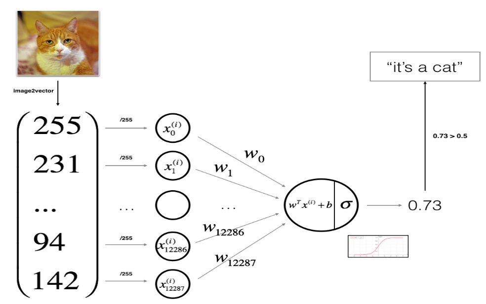
数学表达上述网络：
一个栗子，对于x ( i ) x^{(i)}x (i )：
z ( i ) = w T x ( i ) + b y ^ ( i ) = a ( i ) = sigmoid ⁡ ( z ( i ) ) L ( a ( i ) , y ( i ) ) = − y ( i ) log ⁡ ( a ( i ) ) − ( 1 − y ( i ) ) log ⁡ ( 1 − a ( i ) ) \begin{gathered} z^{(i)}=w^{T} x^{(i)}+b \ \hat{y}^{(i)}=a^{(i)}=\operatorname{sigmoid}\left(z^{(i)}\right) \ \mathcal{L}\left(a^{(i)}, y^{(i)}\right)=-y^{(i)} \log \left(a^{(i)}\right)-\left(1-y^{(i)}\right) \log \left(1-a^{(i)}\right) \end{gathered}z (i )=w T x (i )+b y ^​(i )=a (i )=s i g m o i d (z (i ))L (a (i ),y (i ))=−y (i )lo g (a (i ))−(1 −y (i ))lo g (1 −a (i ))​
损失函数（根据所有的训练样本）：
J = 1 m ∑ i = 1 m L ( a ( i ) , y ( i ) ) J=\frac{1}{m} \sum_{i=1}^{m} \mathcal{L}\left(a^{(i)}, y^{(i)}\right)J =m 1 ​i =1 ∑m ​L (a (i ),y (i ))
在后面的练习中，我们也是按照如下步骤：

• Initialize the parameters of the model
• Learn the parameters for the model by minimizing the cost
• Use the learned parameters to make predictions (on the test set)
• Analyse the results and conclude

; 四、构建自己的算法

搭建神经网络的如下主要步骤，并且我们一般将如下步骤组成 model函数：
（1）定义模型结构，如输入的特征个数
（2）初始化模型变量值
（3）循环：
——计算当前的损失函数（forward propagation）
——计算当前的梯度（backward propagation）
——更新parameters（梯度下降）

1.复习Helper函数

正如刚才上面的图所示，需要计算：
sigmoid ⁡ ( w T x + b ) = 1 1 + e − ( u T x + b ) \operatorname{sigmoid}\left(w^{T} x+b\right)=\frac{1}{1+e^{-\left(u^{T} x+b\right)}}s i g m o i d (w T x +b )=1 +e −(u T x +b )1 ​

练习3——sigmoid

def sigmoid(z):
    s = 1 / (1 + np.exp(-z))
    return s

print ("sigmoid([0, 2]) = " + str(sigmoid(np.array([0,2]))))

2.Initializing parameters

练习4——初始化参数为0向量

def initialize_with_zeros(dim):
"""
    This function creates a vector of zeros of shape (dim, 1) for w and initializes b to 0.

    Argument:
    dim -- size of the w vector we want (or number of parameters in this case)

    Returns:
    w -- initialized vector of shape (dim, 1)
    b -- initialized scalar (corresponds to the bias)
"""

    w = np.zeros((dim, 1))
    b = .0

    assert(w.shape == (dim, 1))
    assert(isinstance(b, float) or isinstance(b, int))

    return w, b

dim = 2
w, b = initialize_with_zeros(dim)
print ("w = " + str(w))
print ("b = " + str(b))

结果为：

w = [[0.]
 [0.]]
b = 0.0

3.向前传播和向后传播

这步需要学习出参数值

练习5——传播函数propagate计算损失值和梯度

（1）获得X
（2）计算：
A = σ ( w T X + b ) = ( a ( 0 ) , a ( 1 ) , … , a ( m − 1 ) , a ( m ) ) A=\sigma\left(w^{T} X+b\right)=\left(a^{(0)}, a^{(1)}, \ldots, a^{(m-1)}, a^{(m)}\right)A =σ(w T X +b )=(a (0 ),a (1 ),…,a (m −1 ),a (m ))
（3）计算损失函数：
J = − 1 m ∑ i = 1 m y ( i ) log ⁡ ( a ( i ) ) + ( 1 − y ( i ) ) log ⁡ ( 1 − a ( i ) ) J=-\frac{1}{m} \sum_{i=1}^{m} y^{(i)} \log \left(a^{(i)}\right)+\left(1-y^{(i)}\right) \log \left(1-a^{(i)}\right)J =−m 1 ​i =1 ∑m ​y (i )lo g (a (i ))+(1 −y (i ))lo g (1 −a (i ))
ps：有2个式子后面会用到：
∂ J ∂ w = 1 m X ( A − Y ) T ∂ J ∂ b = 1 m ∑ i = 1 m ( a ( i ) − y ( i ) ) \begin{aligned} &\frac{\partial J}{\partial w}=\frac{1}{m} X(A-Y)^{T} \ &\frac{\partial J}{\partial b}=\frac{1}{m} \sum_{i=1}^{m}\left(a^{(i)}-y^{(i)}\right) \end{aligned}​∂w ∂J ​=m 1 ​X (A −Y )T ∂b ∂J ​=m 1 ​i =1 ∑m ​(a (i )−y (i ))​

def propagate(w, b, X, Y):
"""
    Implement the cost function and its gradient for the propagation explained above

    Arguments:
    w -- weights, a numpy array of size (num_px * num_px * 3, 1)
    b -- bias, a scalar
    X -- data of size (num_px * num_px * 3, number of examples)
    Y -- true "label" vector (containing 0 if non-cat, 1 if cat) of size (1, number of examples)

    Return:
    cost -- negative log-likelihood cost for logistic regression
    dw -- gradient of the loss with respect to w, thus same shape as w
    db -- gradient of the loss with respect to b, thus same shape as b

    Tips:
    - Write your code step by step for the propagation. np.log(), np.dot()
"""

    m = X.shape[1]

    A = sigmoid(np.dot(w.T, X) + b)
    cost = -1 / m * np.sum(np.dot(Y, np.log(A).T) + np.dot((1 - Y), np.log(1 - A).T))

    dw = 1 / m * np.dot(X, (A - Y).T)
    db = 1 / m * np.sum((A - Y))

    assert(dw.shape == w.shape)
    assert(db.dtype == float)
    cost = np.squeeze(cost)
    assert(cost.shape == ())

    grads = {"dw": dw,
             "db": db}

    return grads, cost

w, b, X, Y = np.array([[1],[2]]), 2, np.array([[1,2],[3,4]]), np.array([[1,0]])
grads, cost = propagate(w, b, X, Y)
print ("dw = " + str(grads["dw"]))
print ("db = " + str(grads["db"]))
print ("cost = " + str(cost))

结果为：

dw = [[0.99993216]
 [1.99980262]]
db = 0.49993523062470574
cost = 6.000064773192205

4.优化器

你已经初始化了参数，也能够用刚才的propagate计算损失函数及其梯度，现在需要更新参数值（用梯度下降）。

练习6——优化optimize

目标是通过使损失函数J最小时学习到w和b参数，更新的表达式为：θ = θ − α d θ , where α is the learning rate. \theta=\theta-\alpha d \theta, \text { where } \alpha \text { is the learning rate. }θ=θ−αd θ,where αis the learning rate.

def optimize(w, b, X, Y, num_iterations, learning_rate, print_cost = False):
"""
    This function optimizes w and b by running a gradient descent algorithm

    Arguments:
    w -- weights, a numpy array of size (num_px * num_px * 3, 1)
    b -- bias, a scalar
    X -- data of shape (num_px * num_px * 3, number of examples)
    Y -- true "label" vector (containing 0 if non-cat, 1 if cat), of shape (1, number of examples)
    num_iterations -- number of iterations of the optimization loop
    learning_rate -- learning rate of the gradient descent update rule
    print_cost -- True to print the loss every 100 steps

    Returns:
    params -- dictionary containing the weights w and bias b
    grads -- dictionary containing the gradients of the weights and bias with respect to the cost function
    costs -- list of all the costs computed during the optimization, this will be used to plot the learning curve.

    Tips:
    You basically need to write down two steps and iterate through them:
        1) Calculate the cost and the gradient for the current parameters. Use propagate().

        2) Update the parameters using gradient descent rule for w and b.

"""

    costs = []

    for i in range(num_iterations):

        grads, cost = propagate(w, b, X, Y)

        dw = grads["dw"]
        db = grads["db"]

        w = w - learning_rate * dw
        b = b - learning_rate * db

        if i % 100 == 0:
            costs.append(cost)

        if print_cost and i % 100 == 0:
            print ("Cost after iteration %i: %f" %(i, cost))

    params = {"w": w,
              "b": b}

    grads = {"dw": dw,
             "db": db}

    return params, grads, costs

params, grads, costs = optimize(w, b, X, Y, num_iterations= 100, learning_rate = 0.009, print_cost = False)

print ("w = " + str(params["w"]))
print ("b = " + str(params["b"]))
print ("dw = " + str(grads["dw"]))
print ("db = " + str(grads["db"]))

输出为：

w = [[0.1124579 ]
 [0.23106775]]
b = 1.5593049248448891
dw = [[0.90158428]
 [1.76250842]]
db = 0.4304620716786828

练习7——预测predict

前面的函数将输出学习到的w和b。我们能够使用w和b预测数据集x的标签。实现predict()函数。计算预测有两个步骤:
Y ^ = A = σ ( w T X + b ) \hat{Y}=A=\sigma\left(w^{T} X+b\right)Y ^=A =σ(w T X +b )然后将a转换为0(如果a c t i v a t i o n activation a c t i v a t i o n激活

def predict(w, b, X):
    '''
    Predict whether the label is 0 or 1 using learned logistic regression parameters (w, b)

    Arguments:
    w -- weights, a numpy array of size (num_px * num_px * 3, 1)
    b -- bias, a scalar
    X -- data of size (num_px * num_px * 3, number of examples)

    Returns:
    Y_prediction -- a numpy array (vector) containing all predictions (0/1) for the examples in X
    '''

    m = X.shape[1]
    Y_prediction = np.zeros((1,m))
    w = w.reshape(X.shape[0], 1)

    A = sigmoid(np.dot(w.T, X) + b)

    for i in range(A.shape[1]):

        if A[0, i]  0.5:
            Y_prediction[0, i] = 0
        elif A[0, i] > 0.5:
            Y_prediction[0, i] = 1

    assert(Y_prediction.shape == (1, m))

    return Y_prediction

print ("predictions = " + str(predict(w, b, X)))

已经实现了几个函数:

• 初始化(w,b)
• 迭代地优化损失以学习参数(w,b):
• 计算代价及其梯度
• 使用梯度下降更新参数
• 使用学习到的(w,b)来预测给定一组示例的标签

五、将所有的函数合并成一个模型

• Y_prediction用于测试集上的预测
• Y_prediction_train用于训练集上的预测
• w, cost, gradient用于optimize()函数的输出

练习8——合成model

def model(X_train, Y_train, X_test, Y_test, num_iterations = 2000, learning_rate = 0.5, print_cost = False):
"""
    Builds the logistic regression model by calling the function you've implemented previously

    Arguments:
    X_train -- training set represented by a numpy array of shape (num_px * num_px * 3, m_train)
    Y_train -- training labels represented by a numpy array (vector) of shape (1, m_train)
    X_test -- test set represented by a numpy array of shape (num_px * num_px * 3, m_test)
    Y_test -- test labels represented by a numpy array (vector) of shape (1, m_test)
    num_iterations -- hyperparameter representing the number of iterations to optimize the parameters
    learning_rate -- hyperparameter representing the learning rate used in the update rule of optimize()
    print_cost -- Set to true to print the cost every 100 iterations

    Returns:
    d -- dictionary containing information about the model.

"""

    w, b = initialize_with_zeros(X_train.shape[0])

    parameters, grads, costs = optimize(w, b, X_train, Y_train, num_iterations, learning_rate, print_cost)

    w = parameters["w"]
    b = parameters["b"]

    Y_prediction_test = predict(w, b, X_test)
    Y_prediction_train = predict(w, b, X_train)

    print("train accuracy: {} %".format(100 - np.mean(np.abs(Y_prediction_train - Y_train)) * 100))
    print("test accuracy: {} %".format(100 - np.mean(np.abs(Y_prediction_test - Y_test)) * 100))

    d = {"costs": costs,
         "Y_prediction_test": Y_prediction_test,
         "Y_prediction_train" : Y_prediction_train,
         "w" : w,
         "b" : b,
         "learning_rate" : learning_rate,
         "num_iterations": num_iterations}

    return d

d = model(train_set_x, train_set_y, test_set_x, test_set_y, num_iterations = 2000, learning_rate = 0.005, print_cost = True)

可以看到如下的迭代中的损失函数值：

Cost after iteration 0: 0.693147
Cost after iteration 100: 0.584508
Cost after iteration 200: 0.466949
Cost after iteration 300: 0.376007
Cost after iteration 400: 0.331463
Cost after iteration 500: 0.303273
Cost after iteration 600: 0.279880
Cost after iteration 700: 0.260042
Cost after iteration 800: 0.242941
Cost after iteration 900: 0.228004
Cost after iteration 1000: 0.214820
Cost after iteration 1100: 0.203078
Cost after iteration 1200: 0.192544
Cost after iteration 1300: 0.183033
Cost after iteration 1400: 0.174399
Cost after iteration 1500: 0.166521
Cost after iteration 1600: 0.159305
Cost after iteration 1700: 0.152667
Cost after iteration 1800: 0.146542
Cost after iteration 1900: 0.140872
train accuracy: 99.04306220095694 %
test accuracy: 70.0 %

由上面结果：
训练准确率接近100%。这是一个很好的完整性检查：模型有足够的容量来匹配训练数据。测试错误为68%。考虑到我们使用的数据集很小，而且逻辑回归是一个线性分类器，对于这个简单的模型来说，它实际上是不错的。后面建立一个更好的分类器。

上面的模型显然是过度拟合训练数据。如何减少过拟合——例如使用正则化。使用下面的代码(并更改索引变量)，可以查看测试集图片上的预测。

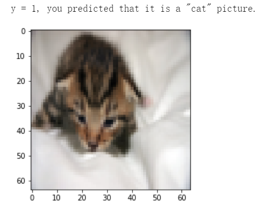
index = 1
plt.imshow(test_set_x[:,index].reshape((num_px, num_px, 3)))
print ("y = " + str(test_set_y[0,index]) + ", you predicted that it is a \"" + classes[int(d["Y_prediction_test"][0,index])].decode("utf-8") +  "\" picture.")

可视化损失函数和梯度：

costs = np.squeeze(d['costs'])
plt.plot(costs)
plt.ylabel('cost')
plt.xlabel('iterations (per hundreds)')
plt.title("Learning rate =" + str(d["learning_rate"]))
plt.show()

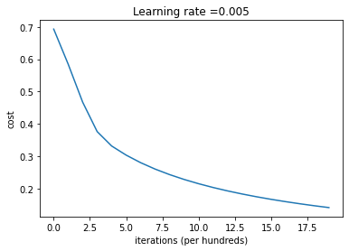
由上图可以看出损失函数在下降，说明参数正在被学习。可以在训练集中训练更多的模型，可以试试增大迭代次数，将会看到训练集的准确率提升，但是测试集的准确率下降——过拟合。

让我们将模型的学习曲线与几种学习速率的选择进行比较。也可以尝试不同的值，而不是我们初始化learning_rates变量要包含的三个值。

六、拓展分析

学习速率𝛼决定了我们更新参数的速度。如果学习率太大，我们可能会”超过”最优值。类似地，如果它太小，我们将需要太多的迭代来收敛到最佳值。

learning_rates = [0.01, 0.001, 0.0001]
models = {}
for i in learning_rates:
    print ("learning rate is: " + str(i))
    models[str(i)] = model(train_set_x, train_set_y, test_set_x, test_set_y, num_iterations = 1500, learning_rate = i, print_cost = False)
    print ('\n' + "-------------------------------------------------------" + '\n')

for i in learning_rates:
    plt.plot(np.squeeze(models[str(i)]["costs"]), label= str(models[str(i)]["learning_rate"]))

plt.ylabel('cost')
plt.xlabel('iterations')

legend = plt.legend(loc='upper center', shadow=True)
frame = legend.get_frame()
frame.set_facecolor('0.90')
plt.show()

数据为：

`python
learning rate is: 0.01
train accuracy: 99.52153110047847 %
test accuracy: 68.0 %

learning rate is: 0.0001
train accuracy: 68.42105263157895 %
test accuracy: 36.0 %

Original: https://blog.csdn.net/qq_35812205/article/details/118816002
Author: 山顶夕景
Title: 【李宏毅机器学习CP9】(task3下)PM2.5预测+numpy实现神经网络logistic回归