

1. 问题和数据
在本练习中,您将使用支持向量机(svm)构建一个垃圾邮件分类器。
在本练习的前半部分,您将使用支持向量机(svm)处理各种示例2D数据集。使用这些数据集进行试验将帮助您直观地了解支持向量机的工作方式,以及如何在支持向量机中使用高斯核。
在练习的下一部分中,您将使用支持向量机构建一个垃圾邮件分类器
对于线性可分案例,我们的任务是找到一条最佳的决策边界,使得离这条决策边界最近的点到该决策边界的距离最远,即为要有最大间隔。


损失函数公式如下:

在本节中要用到新的库,scikit-learn,简称sklearn。可以进行数据的预处理以及最后算法的评估。

; 2.线性可分案例
导入包,numpy和pandas是做运算的库,matplotlib是画图的库。
数据集是在MATLAB的格式,所以要加载它在Python,我们需要使用一个SciPy工具。
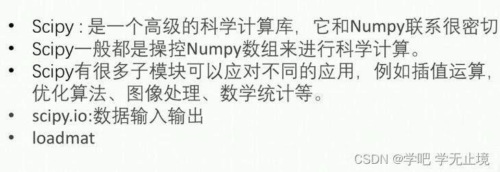
import numpy as np
import scipy.io as sio
import matplotlib.pyplot as plt
导入数据集
data = sio.loadmat('ex6data1.mat')
print('data.keys():', data.keys())
输出结果:
data.keys(): dict_keys(['__header__', '__version__', '__globals__', 'X', 'y'])
指定X, y, 打印shape来看看
X, y = data['X'], data['y']
print('X.shape, y.shape:', X.shape, y.shape)
print('X:', X)
print('y:', y)
输出shape和X,y
X.shape, y.shape: (51, 2) (51, 1)
X: [[1.9643   4.5957  ]
 [2.2753   3.8589  ]
 [2.9781   4.5651  ]
 [2.932    3.5519  ]
 [3.5772   2.856   ]
 [4.015    3.1937  ]
 [3.3814   3.4291  ]
 [3.9113   4.1761  ]
 [2.7822   4.0431  ]
 [2.5518   4.6162  ]
 [3.3698   3.9101  ]
 [3.1048   3.0709  ]
 [1.9182   4.0534  ]
 [2.2638   4.3706  ]
 [2.6555   3.5008  ]
 [3.1855   4.2888  ]
 [3.6579   3.8692  ]
 [3.9113   3.4291  ]
 [3.6002   3.1221  ]
 [3.0357   3.3165  ]
 [1.5841   3.3575  ]
 [2.0103   3.2039  ]
 [1.9527   2.7843  ]
 [2.2753   2.7127  ]
 [2.3099   2.9584  ]
 [2.8283   2.6309  ]
 [3.0473   2.2931  ]
 [2.4827   2.0373  ]
 [2.5057   2.3853  ]
 [1.8721   2.0577  ]
 [2.0103   2.3546  ]
 [1.2269   2.3239  ]
 [1.8951   2.9174  ]
 [1.561    3.0709  ]
 [1.5495   2.6923  ]
 [1.6878   2.4057  ]
 [1.4919   2.0271  ]
 [0.962    2.682   ]
 [1.1693   2.9276  ]
 [0.8122   2.9992  ]
 [0.9735   3.3881  ]
 [1.25     3.1937  ]
 [1.3191   3.5109  ]
 [2.2292   2.201   ]
 [2.4482   2.6411  ]
 [2.7938   1.9656  ]
 [2.091    1.6177  ]
 [2.5403   2.8867  ]
 [0.9044   3.0198  ]
 [0.76615  2.5899  ]
 [0.086405 4.1045  ]]
y: [[1]
 [1]
 [1]
 [1]
 [1]
 [1]
 [1]
 [1]
 [1]
 [1]
 [1]
 [1]
 [1]
 [1]
 [1]
 [1]
 [1]
 [1]
 [1]
 [1]
 [0]
 [0]
 [0]
 [0]
 [0]
 [0]
 [0]
 [0]
 [0]
 [0]
 [0]
 [0]
 [0]
 [0]
 [0]
 [0]
 [0]
 [0]
 [0]
 [0]
 [0]
 [0]
 [0]
 [0]
 [0]
 [0]
 [0]
 [0]
 [0]
 [0]
 [1]]
画出数据的散点图来看看分布状况
def plot_data():
    plt.scatter(X[:, 0], X[:, 1], c=y.flatten(), cmap='jet')

    plt.xlabel('x1')
    plt.ylabel('y1')
    plt.show()

plot_data()

导入sklearn.svm,
from sklearn.svm import SVC
SVC的用法如下:

使用sklearn.svm的svc进行求解
svc1 = SVC(C=1, kernel='linear')
svc1.fit(X, y.flatten())
print(svc1)
print(svc1.predict(X))
print(svc1.score(X, y.flatten()))
打印svc1、预测结果和准确率;当前预测的准确率为0.90039
SVC(C=1, kernel='linear')
[1 1 1 1 1 1 1 1 1 1 1 1 1 1 1 1 1 1 1 1 0 0 0 0 0 0 0 0 0 0 0 0 0 0 0 0 0
 0 0 0 0 0 0 0 0 0 0 0 0 0 0]
0.9803921568627451
绘制决策边界
def plot_boundary(model):
    x_min, x_max = -0.5, 4.5
    y_min, y_max = 1.3, 5
    xx, yy = np.meshgrid(np.linspace(x_min, x_max, 500), np.linspace(y_min, y_max, 500))

    z = model.predict(np.c_[xx.flatten(), yy.flatten()])

    zz = z.reshape(xx.shape)
    plt.contour(xx, yy, zz)

plot_boundary(svc1)
plot_data()
plt.show()

可以看出C=1时有一个样本点是被错分的
接下来我们换一个C的值来看看预测效果
svc100 = SVC(C=100, kernel='linear')
svc100.fit(X, y.flatten())
print(svc100.predict(X))
print(svc100.score(X, y.flatten()))
输出预测结果和准确率:
[1 1 1 1 1 1 1 1 1 1 1 1 1 1 1 1 1 1 1 1 0 0 0 0 0 0 0 0 0 0 0 0 0 0 0 0 0
 0 0 0 0 0 0 0 0 0 0 0 0 0 1]
1.0
调用边界函数画出C=100时的决策边界
plot_boundary(svc100)
plot_data()
plt.show()

这回原本被分错的点也被正确分类了,但是这样其实有点不太好,可能会出现过拟合?只是我们当前的数据点太少,看不出来。
完整代码:
"""
Created on Sat June 23 15:06:11 2022
@author: wzj
python version: python 3.9

Title: 支持向量机(Support Vector Machines)

案例:使用支持向量机(svm)构建一个垃圾邮件分类器。

数据集:数据文件是ex6data1.mat
"""

import numpy as np
import scipy.io as sio
import matplotlib.pyplot as plt

data = sio.loadmat('ex6data1.mat')
print('data.keys():', data.keys())

X, y = data['X'], data['y']
print('X.shape, y.shape:', X.shape, y.shape)
print('X:', X)
print('y:', y)

def plot_data():
    plt.scatter(X[:, 0], X[:, 1], c=y.flatten(), cmap='jet')

    plt.xlabel('x1')
    plt.ylabel('y1')
    plt.show()

from sklearn.svm import SVC
svc1 = SVC(C=1, kernel='linear')
svc1.fit(X, y.flatten())
print(svc1)
print(svc1.predict(X))
print(svc1.score(X, y.flatten()))

def plot_boundary(model):
    x_min, x_max = -0.5, 4.5
    y_min, y_max = 1.3, 5
    xx, yy = np.meshgrid(np.linspace(x_min, x_max, 500), np.linspace(y_min, y_max, 500))

    z = model.predict(np.c_[xx.flatten(), yy.flatten()])

    zz = z.reshape(xx.shape)
    plt.contour(xx, yy, zz)

plot_boundary(svc1)
plot_data()
plt.show()

svc100 = SVC(C=100, kernel='linear')
svc100.fit(X, y.flatten())
print(svc100.predict(X))
print(svc100.score(X, y.flatten()))

plot_boundary(svc100)
plot_data()
plt.show()
3.线性不可分案例
我们在之前面对线性不可分时用的方法都是建立特征多项式,通过把低维的变量映射到高维,就有可能变成可分的。
而在本次中,我们使用核函数,它的原理也和之前差不多的,可以自动将低维空间映射到高维空间,可以在低微空间计算出高维空间的点积结果(后半句不太明白啥意思,先不管)。

常用的核函数有多项式核,高斯核,拉普拉斯核等,如下 所示。本次会使用的是高斯核。在高斯核中,会有一个叫σ \sigma σ的参数(可能我看的讲解的视频的作者叫错了,叫它gamma),gamma对模型复杂度的影响如下 ,我们之后会通过调整gamma的大小来观察对模型的影响情况。

首先导入库
import numpy as np
import scipy.io as sio
import matplotlib.pyplot as plt
导入数据集,打印表头看看
data = sio.loadmat('ex6data2.mat')
print('data.keys():', data.keys())
输出表头
data.keys(): dict_keys(['__header__', '__version__', '__globals__', 'X', 'y'])
获取X,y,并打印shape来看看
X, y = data['X'], data['y']
print('X.shape, y.shape:', X.shape, y.shape)
输出X,y的shape
X.shape, y.shape: (863, 2) (863, 1)
画出数据的散点图来看看分布状况
def plot_data():
    plt.scatter(X[:, 0], X[:, 1], c=y.flatten(), cmap='jet')

    plt.xlabel('x1')
    plt.ylabel('y1')
    plt.show()

plot_data()
输出散点图:

导入sklearn.svm的库
from sklearn.svm import SVC
调用SVC进行模型预测
svc1 = SVC(C=1, kernel='rbf', gamma=1)

svc1.fit(X, y.flatten())
print(svc1.score(X, y.flatten()))
输出准确率,当前预测的准确率为0.8088064889918888
0.8088064889918888
绘制决策边界
def plot_boundary(model):
    x_min, x_max = 0, 1.0
    y_min, y_max = 0.4, 1.0
    xx, yy = np.meshgrid(np.linspace(x_min, x_max, 500), np.linspace(y_min, y_max, 500))

    z = model.predict(np.c_[xx.flatten(), yy.flatten()])

    zz = z.reshape(xx.shape)
    plt.contour(xx, yy, zz)

plot_boundary(svc1)
plot_data()
plt.show()
绘制出gamma=1时散点图和决策边界图像:
可以看出,当前还不能很好的区分数据点。
我们把上面的gamma=1换成gamma=50:
svc1 = SVC(C=1, kernel=’rbf’, gamma=50)
绘制出gamma=50时的散点图和决策边界图像:
从图中可以看出目前准确率提高了不少,但仍存在一些点不能被区分;并且此时打印出的准确率也达到了0.9895712630359212
0.9895712630359212
我们再把上面的gamma=50换成gamma=1000:
svc1 = SVC(C=1, kernel=’rbf’, gamma=1000)
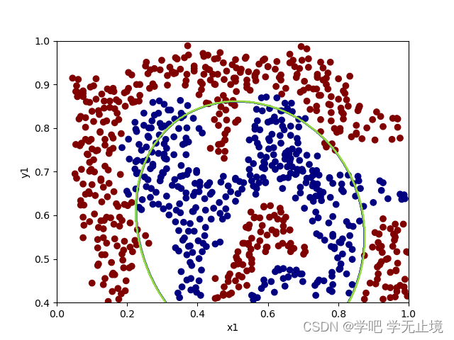
此时模型复杂了很多,绘制出gamma=1000时的散点图和决策边界图像:

从图中可以看出目前准确率又得到提高了,每一个数据点都得到了正确的分类,并且此时打印出的准确率也达到了1.0
1.0
完整代码:
"""
Created on Sat June 23 18:01:23 2022
@author: wzj
python version: python 3.9

Title: 支持向量机(Support Vector Machines)——线性不可分案例

案例:使用支持向量机(svm)构建一个垃圾邮件分类器。

数据集:数据文件是ex6data2.mat
"""

import numpy as np
import scipy.io as sio
import matplotlib.pyplot as plt

data = sio.loadmat('ex6data2.mat')
print('data.keys():', data.keys())

X, y = data['X'], data['y']
print('X.shape, y.shape:', X.shape, y.shape)

def plot_data():
    plt.scatter(X[:, 0], X[:, 1], c=y.flatten(), cmap='jet')

    plt.xlabel('x1')
    plt.ylabel('y1')
    plt.show()

from sklearn.svm import SVC

svc1 = SVC(C=1, kernel='rbf', gamma=1000)

svc1.fit(X, y.flatten())
print(svc1.score(X, y.flatten()))

def plot_boundary(model):
    x_min, x_max = 0, 1.0
    y_min, y_max = 0.4, 1.0
    xx, yy = np.meshgrid(np.linspace(x_min, x_max, 500), np.linspace(y_min, y_max, 500))

    z = model.predict(np.c_[xx.flatten(), yy.flatten()])

    zz = z.reshape(xx.shape)
    plt.contour(xx, yy, zz)

plot_boundary(svc1)
plot_data()
plt.show()
4.寻找最优参数C和gamma
通过前面两个小练习我们已经知道了误差惩罚系数C和高斯核的参数gamma都会对模型精度产生影响,下面我们就来寻找一下最优参数C和gamma的组合方式。
首先导入库
import numpy as np
import scipy.io as sio
import matplotlib.pyplot as plt
from sklearn.svm import SVC
导入数据集,打印表头看看
data = sio.loadmat('ex6data3.mat')
print('data.keys():', data.keys())
输出表头;可以看出这次X,y除了训练集还有验证集;我们将在训练集上进行模型训练,然后到验证集上对模型进行验证
data.keys(): dict_keys(['__header__', '__version__', '__globals__', 'X', 'y', 'yval', 'Xval'])
获取X,y,Xval, yval;并打印X, y的shape来看看
X, y = data['X'], data['y']
Xval, yval = data['Xval'], data['yval']
print('X.shape, y.shape:', X.shape, y.shape)
输出X,y的shape
X.shape, y.shape: (211, 2) (211, 1)
画出数据的散点图来看看分布状况
def plot_data():
    plt.scatter(X[:, 0], X[:, 1], c=y.flatten(), cmap='jet')

    plt.xlabel('x1')
    plt.ylabel('y1')
    plt.show()

plot_data()
输出散点图:

寻找准确率最高时候的最优参数C和gamma
Cvalues = [0.01, 0.03, 0.1, 0.3, 1, 3, 10, 30, 100]
gammas = [0.01, 0.03, 0.1, 0.3, 1, 3, 10, 30, 100]

best_score = 0
best_params = (0, 0)

for c in Cvalues:
    for gamma in gammas:
        svc = SVC(C=c, kernel='rbf', gamma=gamma)
        svc.fit(X, y.flatten())
        score = svc.score(Xval, yval.flatten())
        if score > best_score:
            best_score = score
            best_params = (c, gamma)
print('best_score, best_params:', best_score, best_params)
输出最优准确率为0.965,最优参数C和gamma分别为0.3和100
best_score, best_params: 0.965 (0.3, 100)
将最优参数代回去,得到最后的最优分类图像
svc2 = SVC(C=best_params[0], kernel='rbf', gamma=best_params[1])
svc2.fit(X, y.flatten())
绘制决策边界
def plot_boundary(model):
    x_min, x_max = -0.6, 0.4
    y_min, y_max = -0.7, 0.7
    xx, yy = np.meshgrid(np.linspace(x_min, x_max, 500), np.linspace(y_min, y_max, 500))

    z = model.predict(np.c_[xx.flatten(), yy.flatten()])

    zz = z.reshape(xx.shape)
    plt.contour(xx, yy, zz)

plot_boundary(svc2)
plot_data()
plt.show()

最高的预测率best_score确实是0.965,但是能达到这个预测率的best_params其实不止有(0.3, 100)这一组,只是按照我们设置的遍历和赋值的特点,他们恰好是最靠后的一组。
完整代码:
"""
Created on Sat June 23 18:01:23 2022
@author: wzj
python version: python 3.9

Title: 支持向量机(Support Vector Machines)——寻找最优参数C和gamma

案例:使用支持向量机(svm)构建一个垃圾邮件分类器。

数据集:数据文件是ex6data3.mat
"""

import numpy as np
import scipy.io as sio
import matplotlib.pyplot as plt
from sklearn.svm import SVC

data = sio.loadmat('ex6data3.mat')
print('data.keys():', data.keys())

X, y = data['X'], data['y']
Xval, yval = data['Xval'], data['yval']
print('X.shape, y.shape:', X.shape, y.shape)

def plot_data():
    plt.scatter(X[:, 0], X[:, 1], c=y.flatten(), cmap='jet')

    plt.xlabel('x1')
    plt.ylabel('y1')
    plt.show()

Cvalues = [0.01, 0.03, 0.1, 0.3, 1, 3, 10, 30, 100]
gammas = [0.01, 0.03, 0.1, 0.3, 1, 3, 10, 30, 100]

best_score = 0
best_params = (0, 0)

for c in Cvalues:
    for gamma in gammas:
        svc = SVC(C=c, kernel='rbf', gamma=gamma)
        svc.fit(X, y.flatten())
        score = svc.score(Xval, yval.flatten())
        if score > best_score:
            best_score = score
            best_params = (c, gamma)
print('best_score, best_params:', best_score, best_params)

svc2 = SVC(C=best_params[0], kernel='rbf', gamma=best_params[1])
svc2.fit(X, y.flatten())

def plot_boundary(model):
    x_min, x_max = -0.6, 0.4
    y_min, y_max = -0.7, 0.7
    xx, yy = np.meshgrid(np.linspace(x_min, x_max, 500), np.linspace(y_min, y_max, 500))

    z = model.predict(np.c_[xx.flatten(), yy.flatten()])

    zz = z.reshape(xx.shape)
    plt.contour(xx, yy, zz)

plot_boundary(svc2)
plot_data()
plt.show()
5.通过SVM判断一封邮件是否是垃圾邮件
首先导入库
import numpy as np
import scipy.io as sio
import matplotlib.pyplot as plt
from sklearn.svm import SVC
导入训练集数据和测试集数据,打印表头看看
data1 = sio.loadmat('spamTrain.mat')
print('data1.keys():', data1.keys())

data2 = sio.loadmat('spamTest.mat')
print('data2.keys():', data2.keys())
输出表头;可以看出这次X,y除了训练集还有验证集;我们将在训练集上进行模型训练,然后到验证集上对模型进行验证
data1.keys(): dict_keys(['__header__', '__version__', '__globals__', 'X', 'y'])
data2.keys(): dict_keys(['__header__', '__version__', '__globals__', 'Xtest', 'ytest'])
获取X,y,Xtest, ytest ;并打印X, y的shape以及X,y来看看
X, y = data1['X'], data1['y']
Xtest, ytest = data2['Xtest'], data2['ytest']
print('X.shape, y.shape:', X.shape, y.shape)
print('X:', X)
print('y:', y)
输出X,y的shape
X由1899种特征来表示,这些特征由0和1组成,0表示语义库不能找到该单词,1表示语义库可以找到该单
y只有0和1两种形式,1表示当前邮件为垃圾邮件,0表示不是垃圾邮件
X.shape, y.shape: (4000, 1899) (4000, 1)
X: [[0 0 0 ... 0 0 0]
 [0 0 0 ... 0 0 0]
 [0 0 0 ... 0 0 0]
 ...

 [0 0 0 ... 0 0 0]
 [0 0 1 ... 0 0 0]
 [0 0 0 ... 0 0 0]]
y: [[1]
 [1]
 [0]
 ...

 [1]
 [0]
 [0]]
调用SVC进行邮件分类, 打印出最好的分数结果best_score与其对应的参数best_param
Cvalues = [3, 10, 30, 100, 0.01, 0.03, 0.1, 0.3, 1]
best_score = 0
best_param = 0

for c in Cvalues:
    svc = SVC(C=c, kernel='linear')
    svc.fit(X, y.flatten())
    score = svc.score(Xtest, ytest.flatten())
    if score > best_score:
        best_score = score
        best_param = c

print('best_score, best_param:', best_score, best_param)
输出最好的分数结果best_score与其对应的参数best_param:
best_score, best_param: 0.99 0.03
将最优的参数best_param分别带入训练集和测试集,得到在各自数据下的最好分数(预测准确率)
svc = SVC(C= best_param, kernel='linear')
svc.fit(X, y.flatten())
score_train = svc.score(X, y.flatten())
score_test = svc.score(Xtest, ytest.flatten())
print('score_train, score_test:', best_score, best_param)
分别输出代入最优参数best_param=0.03时,在测试集和验证集上得到的最优的分数结果,
在训练集上的预测准确率为0.99,在验证集上的预测准确率也为0.99。
best_score, best_param: 0.99 0.03
score_train, score_test: 0.99 0.03
参考文献:
[1] https://www.bilibili.com/video/BV1xJ411U7g9?p=5&spm_id_from=pageDriver&vd_source=72e4369cf6b54497a1e04f2071a47a1e
Original: https://blog.csdn.net/weixin_46915208/article/details/125427559
Author: 学吧 学无止境
Title: 吴恩达机器学习课后作业6——使用支持向量机(svm)构建一个垃圾邮件分类器
原创文章受到原创版权保护。转载请注明出处:https://www.johngo689.com/721012/
转载文章受原作者版权保护。转载请注明原作者出处!