

很多场景下,我们需要将信号进行分解,为我们下一步操作提供方便,常用的分解方法可以有EMD族类,例如EMD、EEMD、FEEMD、CEEMDAN、ICEEMDAN等,当然也有小波分解、经验小波分解等,总之分解方式多种多样,根据样本的特点,选用不同的分解方式。这里简要介绍VMD分解。
Konstantin等人在2014年提出了一个完全非递归的(VMD)它可以实现分解模态的同时提取。该模型寻找一组模态和它们各自的中心频率,以便这些模态共同再现输入信号,同时每个模态在解调到基带后都是平滑的。算法的本质是将经典的维纳滤波器推广到多个自适应波段,使得其具有坚实的理论基础,并且容易理解。采用交替方向乘子法对变分模型进行有效优化,使得模型对采样噪声的鲁棒性更强。
VMD分解的具体过程可以理解为变分问题的最优解,可以相应转化为变分问题的构造和求解。


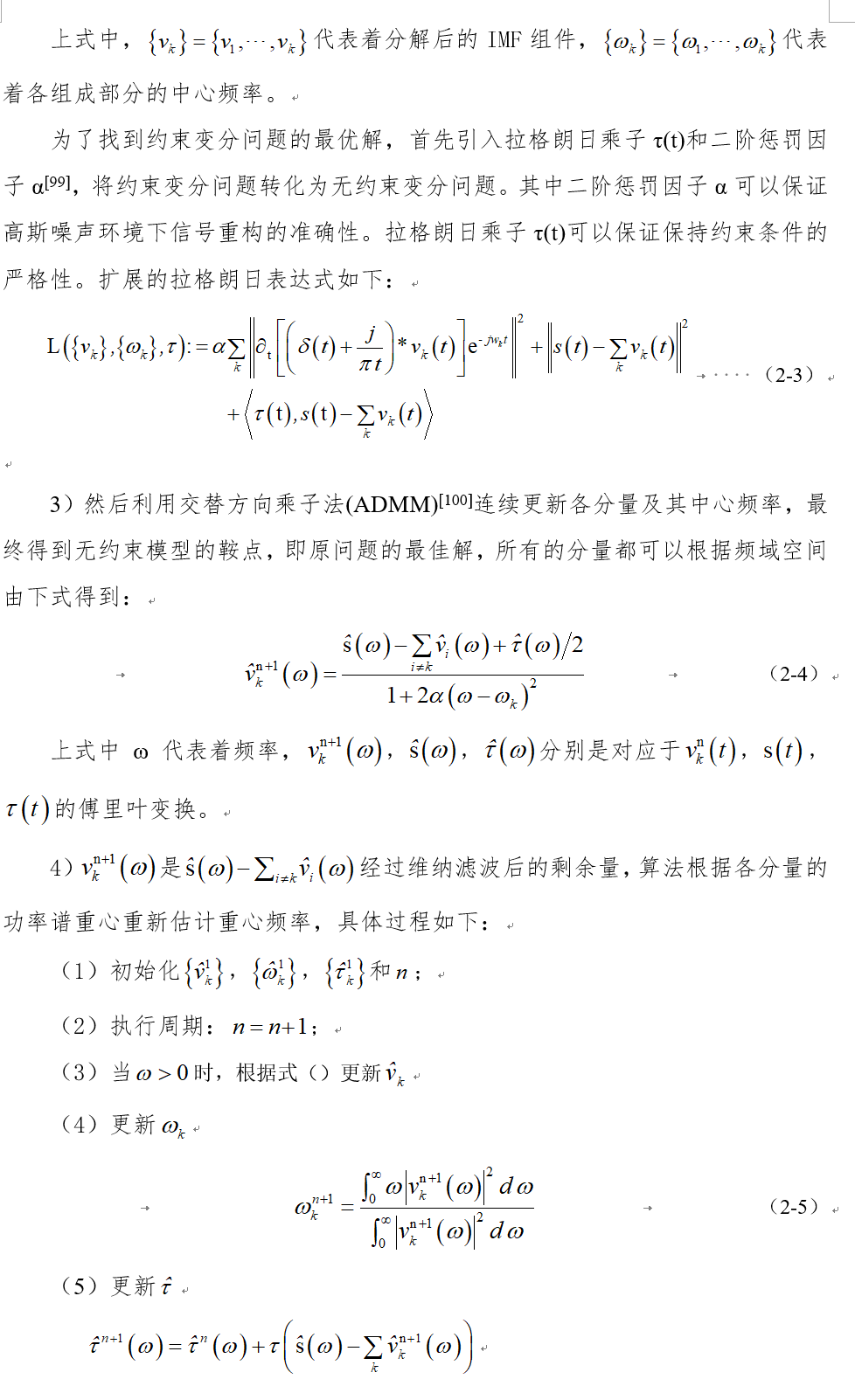
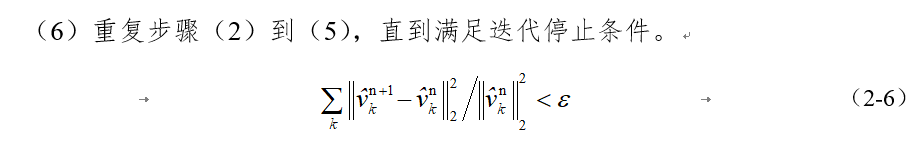
以上就是VMD(变分模态分解)的理论部分,大家不一定全弄明白,因为本人看了原文,也不能完全弄懂里面的数学关系。大体知道分解的过程包含哪几个步骤即可,知网上面关于这类分解的文章也很多,大家可以参考浏览学习下。
下面直接上代码。
function [u, u_hat, omega] = VMD(signal, alpha, tau, K, DC, init, tol)
% Variational Mode Decomposition
% Authors: Konstantin Dragomiretskiy and Dominique Zosso
% zosso@math.ucla.edu --- http://www.math.ucla.edu/~zosso
% Initial release 2013-12-12 (c) 2013
%
% Input and Parameters:
% ---------------------
% signal  - the time domain signal (1D) to be decomposed
% alpha   - the balancing parameter of the data-fidelity constraint
% tau     - time-step of the dual ascent ( pick 0 for noise-slack )
% K       - the number of modes to be recovered
% DC      - true if the first mode is put and kept at DC (0-freq)
% init    - 0 = all omegas start at 0
%                    1 = all omegas start uniformly distributed
%                    2 = all omegas initialized randomly
% tol     - tolerance of convergence criterion; typically around 1e-6
%
% Output:
% -------
% u       - the collection of decomposed modes
% u_hat   - spectra of the modes
% omega   - estimated mode center-frequencies
%
% When using this code, please do cite our paper:
% -----------------------------------------------
% K. Dragomiretskiy, D. Zosso, Variational Mode Decomposition, IEEE Trans.

% on Signal Processing (in press)
% please check here for update reference:
%          http://dx.doi.org/10.1109/TSP.2013.2288675

%---------- Preparations

% Period and sampling frequency of input signal
save_T = length(signal);
fs = 1/save_T;

% extend the signal by mirroring
T = save_T;
f_mirror(1:T/2) = signal(T/2:-1:1);
f_mirror(T/2+1:3*T/2) = signal;
f_mirror(3*T/2+1:2*T) = signal(T:-1:T/2+1);
f = f_mirror;

% Time Domain 0 to T (of mirrored signal)
T = length(f);
t = (1:T)/T;

% Spectral Domain discretization
freqs = t-0.5-1/T;

% Maximum number of iterations (if not converged yet, then it won't anyway)
N = 500;

% For future generalizations: individual alpha for each mode
Alpha = alpha*ones(1,K);

% Construct and center f_hat
f_hat = fftshift((fft(f)));
f_hat_plus = f_hat;
f_hat_plus(1:T/2) = 0;

% matrix keeping track of every iterant // could be discarded for mem
u_hat_plus = zeros(N, length(freqs), K);

% Initialization of omega_k
omega_plus = zeros(N, K);
switch init
    case 1
        for i = 1:K
            omega_plus(1,i) = (0.5/K)*(i-1);
        end
    case 2
        omega_plus(1,:) = sort(exp(log(fs) + (log(0.5)-log(fs))*rand(1,K)));
    otherwise
        omega_plus(1,:) = 0;
end

% if DC mode imposed, set its omega to 0
if DC
    omega_plus(1,1) = 0;
end

% start with empty dual variables
lambda_hat = zeros(N, length(freqs));

% other inits
uDiff = tol+eps; % update step
n = 1; % loop counter
sum_uk = 0; % accumulator

% ----------- Main loop for iterative updates

while ( uDiff > tol &&  n < N ) % not converged and below iterations limit

    % update first mode accumulator
    k = 1;
    sum_uk = u_hat_plus(n,:,K) + sum_uk - u_hat_plus(n,:,1);

    % update spectrum of first mode through Wiener filter of residuals
    u_hat_plus(n+1,:,k) = (f_hat_plus - sum_uk - lambda_hat(n,:)/2)./(1+Alpha(1,k)*(freqs - omega_plus(n,k)).^2);

    % update first omega if not held at 0
    if ~DC
        omega_plus(n+1,k) = (freqs(T/2+1:T)*(abs(u_hat_plus(n+1, T/2+1:T, k)).^2)')/sum(abs(u_hat_plus(n+1,T/2+1:T,k)).^2);
    end

    % update of any other mode
    for k=2:K

        % accumulator
        sum_uk = u_hat_plus(n+1,:,k-1) + sum_uk - u_hat_plus(n,:,k);

        % mode spectrum
        u_hat_plus(n+1,:,k) = (f_hat_plus - sum_uk - lambda_hat(n,:)/2)./(1+Alpha(1,k)*(freqs - omega_plus(n,k)).^2);

        % center frequencies
        omega_plus(n+1,k) = (freqs(T/2+1:T)*(abs(u_hat_plus(n+1, T/2+1:T, k)).^2)')/sum(abs(u_hat_plus(n+1,T/2+1:T,k)).^2);

    end

    % Dual ascent
    lambda_hat(n+1,:) = lambda_hat(n,:) + tau*(sum(u_hat_plus(n+1,:,:),3) - f_hat_plus);

    % loop counter
    n = n+1;

    % converged yet?

    uDiff = eps;
    for i=1:K
        uDiff = uDiff + 1/T*(u_hat_plus(n,:,i)-u_hat_plus(n-1,:,i))*conj((u_hat_plus(n,:,i)-u_hat_plus(n-1,:,i)))';
    end
    uDiff = abs(uDiff);

end

%------ Postprocessing and cleanup

% discard empty space if converged early
N = min(N,n);
omega = omega_plus(1:N,:);

% Signal reconstruction
u_hat = zeros(T, K);
u_hat((T/2+1):T,:) = squeeze(u_hat_plus(N,(T/2+1):T,:));
u_hat((T/2+1):-1:2,:) = squeeze(conj(u_hat_plus(N,(T/2+1):T,:)));
u_hat(1,:) = conj(u_hat(end,:));

u = zeros(K,length(t));

for k = 1:K
    u(k,:)=real(ifft(ifftshift(u_hat(:,k))));
end

% remove mirror part
u = u(:,T/4+1:3*T/4);

% recompute spectrum
clear u_hat;
for k = 1:K
    u_hat(:,k)=fftshift(fft(u(k,:)))';
end

end
代码很长,尽量看,能看懂多少看懂多少。这里不再讲解,因为这里都是对数学原理的复现,如果要弄懂原理,建议比照原文和代码相结合,逐行去看。如果只是利用这种分解方式,关心得出的结果,那么就没有必要大费周章了。
function [u, u_hat, omega] = VMD(signal, alpha, tau, K, DC, init, tol)
函数的输入输出,这里要解释一下。
函数的输入部分:signal代表输入信号,alpha表示数据保真度约束的平衡参数 ,tau表示时间步长,K表示分解层数,DC表示如果将第一模式置于DC(0频率),则为true。 init表示信号的初始化,tol表示收敛容错准则。通常除了K,也就是分解模态数之外,其他参数都有相应的经验值。绝大部分文献对VMD的探索也是对分解模态数的确定,顶多再加上tau的讨论。(博主后面的文章中也会进行相应的讨论。)
函数的输出部分:u表示分解模式的集合,u_hat表示模式的光谱范围,omega 表示估计模态的中心频率。
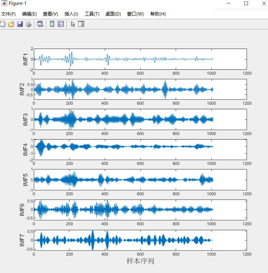
下面是调用VMD分解的主程序。主要步骤就是输入信号值,确定VMD的分解参数,画图。
tic
clc
clear all

load('IMF1_7.mat')
x=IMF1_7;
t=1:length(IMF1_7);

%--------- 对于VMD参数进行设置---------------
alpha = 2000;       % moderate bandwidth constraint:适度的带宽约束/惩罚因子
tau = 0.0244;          % noise-tolerance (no strict fidelity enforcement):噪声容限(没有严格的保真度执行)
K = 7;              % modes:分解的模态数
DC = 0;             % no DC part imposed:无直流部分
init = 1;           % initialize omegas uniformly  :omegas的均匀初始化
tol = 1e-6 ;
%--------------- Run actual VMD code:数据进行vmd分解---------------------------
[u, u_hat, omega] = VMD(x, alpha, tau, K, DC, init, tol);
figure;
imfn=u;
n=size(imfn,1); %size(X,1),返回矩阵X的行数;size(X,2),返回矩阵X的列数;N=size(X,2),就是把矩阵X的列数赋值给N

for n1=1:n
    subplot(n,1,n1);
    plot(t,u(n1,:));%输出IMF分量,a(:,n)则表示矩阵a的第n列元素,u(n1,:)表示矩阵u的n1行元素
    ylabel(['IMF' ,int2str(n1)],'fontsize',11);%int2str(i)是将数值i四舍五入后转变成字符,y轴命名
end
 xlabel('样本序列','fontsize',14,'fontname','宋体');

%时间\itt/s
 toc;
下图记为分解的结果。
以上就是对VMD分解的简单描述,下面的博文中将探讨如何对分解层数进行相应固定。
Original: https://blog.csdn.net/weixin_46062179/article/details/122268070
Author: soap皂
Title: 浅谈VMD—变分模态分解
原创文章受到原创版权保护。转载请注明出处:https://www.johngo689.com/716057/
转载文章受原作者版权保护。转载请注明原作者出处!