可解释性研究 -LRP-for-LSTM

2023年7月23日下午12:09 • 人工智能 • 阅读 46

LRP算法

一.LSTM
*
1.1.理论部分
1.2.作者代码
二.LRP_for_LSTM
*
2.1.理论部分
–
- 2.2.1.Weighted Connections
- 2.2.2.Multiplicative Interactions
2.2.作者代码
三.扩展到GRU
*
3.1.GRU
3.2.GRU的Relevance计算部分
四.参考文献

LRP算法也是可解释算法的一种，全称Layer-wise Relevance Propagation，原始LRP算法主要是应用在CV等领域，针对NLP中通过Word2Vec等手段将token转化为分布式词向量并通过RNN向量化文档的可解释手段真不多。LIME虽然可以针对文本数据进行解释，但适用场景是tf-idf或者bag-of-word这种词向量，向量中一个维度代表一个词。

这里参考的论文是Explaining Recurrent Neural Network Predictions in Sentiment Analysis，作者将LRP算法扩展到LSTM中，这里应用的任务是一个5分类情感任务，输入一个词序列，输出这句话属于哪个类别，LRP算法输出序列中哪几个词是重点。

代码开源到github，但是这里作者用numpy实现了个LSTM，并用LRP解释。如何添加对pytorch，keras框架还没人做过。先来研究下内部实现。

一.LSTM

1.1.理论部分

关于LSTM可以参考LSTM详解，这里为了跟作者的代码同步，再提几句。LSTM大致结构如下

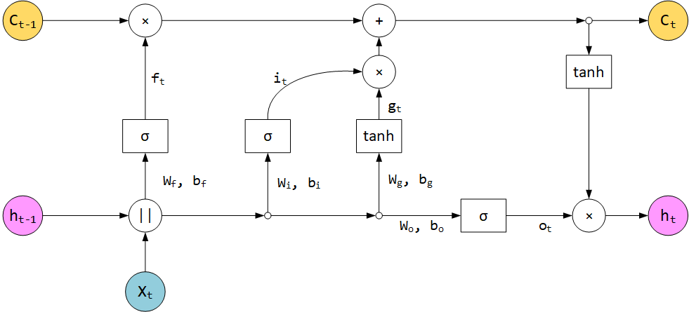
这里模型每一个时间步的输出为 h t h_t h t ，从t – 1时刻到t时刻可以用 C t , h t = L S T M C e l l ( C t − 1 , h t − 1 , x t ) C_t, h_t = LSTMCell(C_{t – 1}, h_{t – 1}, x_t)C t ,h t =L S T M C e l l (C t −1 ,h t −1 ,x t ) 表示，x t x_t x t 是输入向量，W f , W i , W o , W g , b f , b i , b o , b g W_f, W_i, W_o, W_g, b_f, b_i, b_o, b_g W f ,W i ,W o ,W g ,b f ,b i ,b o ,b g 均为模型参数（模型参数写法有很多种，作者代码实现的就有些区别）。

x t ∈ R e x_t \in R^e x t ∈R e
h t ∈ R d h_t \in R^d h t ∈R d
C t ∈ R d C_t \in R^d C t ∈R d
W f , W i , W o , W g ∈ R ( d + e ) × d W_f, W_i, W_o, W_g \in R^{(d + e) \times d}W f ,W i ,W o ,W g ∈R (d +e )×d
b f , b i , b o , b g ∈ R d b_f, b_i, b_o, b_g \in R^d b f ,b i ,b o ,b g ∈R d
f t , i t , g t , o t ∈ R d f_t, i_t, g_t, o_t \in R^d f t ,i t ,g t ,o t ∈R d

上图

∣ ∣ ||∣∣ 表示concat操作，∣ ∣ ( h t − 1 , x t ) = [ h t − 1 ; x t ] ||(h_{t – 1}, x_t) = [h_{t – 1};x_t]∣∣(h t −1 ,x t )=[h t −1 ;x t ]
σ \sigma σ 表示sigmoid，箭头线带2个参数+sigmoid表示σ ( W . [ h t − 1 ; x t ] + b ) \sigma(W.[h_{t – 1};x_t] + b)σ(W .[h t −1 ;x t ]+b )
t a n h tanh t a n h 表示tanh激活函数
- ++ 表示向量加法
× \times × 表示向量乘法，这里相乘的元素都是1维向量，计算结果是对应位置的元素相乘，依旧是1维向量，比如[ 1 , 2 , 3 ] × [ 4 , 5 , 6 ] = [ 4 , 10 , 18 ] [1,2,3] \times [4, 5, 6] = [4, 10, 18][1 ,2 ,3 ]×[4 ,5 ,6 ]=[4 ,1 0 ,1 8 ]

这里就把上面涉及的公式总结下，要是觉得多余了就直接往下翻

f t = σ ( W f . [ h t − 1 ; x t ] + b f ) f_t = \sigma(W_f.[h_{t – 1}; x_t] + b_f)f t =σ(W f .[h t −1 ;x t ]+b f )
i t = σ ( W i . [ h t − 1 ; x t ] + b i ) i_t = \sigma(W_i.[h_{t – 1}; x_t] + b_i)i t =σ(W i .[h t −1 ;x t ]+b i )
g t = t a n h ( W g . [ h t − 1 ; x t ] + b g ) g_t = tanh(W_g.[h_{t – 1}; x_t] + b_g)g t =t a n h (W g .[h t −1 ;x t ]+b g )
o t = σ ( W o . [ h t − 1 ; x t ] + b o ) o_t = \sigma(W_o.[h_{t – 1}; x_t] + b_o)o t =σ(W o .[h t −1 ;x t ]+b o )
C t = C t − 1 × f t + i t × g t C_t = C_{t – 1} \times f_t + i_t \times g_t C t =C t −1 ×f t +i t ×g t
h t = o t × t a n h ( C t ) h_t = o_t \times tanh(C_t)h t =o t ×t a n h (C t )

针对双向LSTM，假设输入序列长度为 T T T，那么最终输出 c c c
c = W l e f t . h l e f t T + W r i g h t . h r i g h t T c = W_{left} . h_{left}^T + W_{right}. h_{right}^T c =W l e f t .h l e f t T +W r i g h t .h r i g h t T

c ∈ R C c \in R^C c ∈R C，C C C 为类别数
W l e f t , W r i g h t ∈ R C × d W_{left}, W_{right} \in R^{C \times d}W l e f t ,W r i g h t ∈R C ×d

; 1.2.作者代码

class LSTM_bidi:
    def __init__(self, model_path='./model/'):
"""
        Load trained model from file.

"""

        f_voc = open(model_path + "vocab", 'rb')
        self.voc  = pickle.load(f_voc)
        f_voc.close()

        self.E    = np.load(model_path + 'embeddings.npy', mmap_mode='r')

        f_model   = open(model_path + 'model', 'rb')
        model     = pickle.load(f_model)
        f_model.close()

        self.Wxh_Left  = model["Wxh_Left"]
        self.bxh_Left  = model["bxh_Left"]
        self.Whh_Left  = model["Whh_Left"]
        self.bhh_Left  = model["bhh_Left"]

        self.Wxh_Right = model["Wxh_Right"]
        self.bxh_Right = model["bxh_Right"]
        self.Whh_Right = model["Whh_Right"]
        self.bhh_Right = model["bhh_Right"]

        self.Why_Left  = model["Why_Left"]
        self.Why_Right = model["Why_Right"]

这里作者实现的是 双向LSTM，一个left，一个right，我们只关注其中一个，left。可以看到作者这里并没有定义concat操作，而是对参数进行了重组，之前的 W f , W i , W g , W o W_f, W_i, W_g, W_o W f ,W i ,W g ,W o 重组成了 W x h W_{xh}W x h 和 W h h W_{hh}W h h ，一个用来与 x t x_t x t 运算一个用来与 h t − 1 h_{t – 1}h t −1 运算。W x h W_{xh}W x h 包括了 W f , W i , W g , W o W_f, W_i, W_g, W_o W f ,W i ,W g ,W o 中与 x t x_t x t 运算的部分而 W h h W_{hh}W h h 包括了与 h t − 1 h_{t – 1}h t −1 运算的部分。

    def forward(self):
"""
        Standard forward pass.

        Compute the hidden layer values (assuming input x/x_rev was previously set)
"""
        print(f"x.shape:{self.x.shape}")
        T = len(self.w)
        d = int(self.Wxh_Left.shape[0]/4)

        idx = np.hstack((np.arange(0,d), np.arange(2*d,4*d))).astype(int)
        idx_i, idx_g, idx_f, idx_o = np.arange(0,d), np.arange(d,2*d), np.arange(2*d,3*d), np.arange(3*d,4*d)

        self.gates_xh_Left = np.zeros((T, 4*d))
        self.gates_hh_Left = np.zeros((T, 4*d))
        self.gates_pre_Left = np.zeros((T, 4*d))
        self.gates_Left = np.zeros((T, 4*d))

        self.gates_xh_Right = np.zeros((T, 4*d))
        self.gates_hh_Right = np.zeros((T, 4*d))
        self.gates_pre_Right= np.zeros((T, 4*d))
        self.gates_Right = np.zeros((T, 4*d))

        for t in range(T):
            self.gates_xh_Left[t] = np.dot(self.Wxh_Left, self.x[t])
            self.gates_hh_Left[t] = np.dot(self.Whh_Left, self.h_Left[t-1])
            self.gates_pre_Left[t] = self.gates_xh_Left[t] + self.gates_hh_Left[t] + self.bxh_Left + self.bhh_Left
            self.gates_Left[t,idx] = 1.0/(1.0 + np.exp(- self.gates_pre_Left[t,idx]))
            self.gates_Left[t,idx_g] = np.tanh(self.gates_pre_Left[t,idx_g])
            self.c_Left[t] = self.gates_Left[t,idx_f]*self.c_Left[t-1] + self.gates_Left[t,idx_i]*self.gates_Left[t,idx_g]
            self.h_Left[t] = self.gates_Left[t,idx_o]*np.tanh(self.c_Left[t])

            self.gates_xh_Right[t] = np.dot(self.Wxh_Right, self.x_rev[t])
            self.gates_hh_Right[t] = np.dot(self.Whh_Right, self.h_Right[t-1])
            self.gates_pre_Right[t] = self.gates_xh_Right[t] + self.gates_hh_Right[t] + self.bxh_Right + self.bhh_Right
            self.gates_Right[t,idx] = 1.0/(1.0 + np.exp(- self.gates_pre_Right[t,idx]))
            self.gates_Right[t,idx_g] = np.tanh(self.gates_pre_Right[t,idx_g])
            self.c_Right[t] = self.gates_Right[t,idx_f]*self.c_Right[t-1] + self.gates_Right[t,idx_i]*self.gates_Right[t,idx_g]
            self.h_Right[t] = self.gates_Right[t,idx_o]*np.tanh(self.c_Right[t])

        self.y_Left  = np.dot(self.Why_Left,  self.h_Left[T-1])
        self.y_Right = np.dot(self.Why_Right, self.h_Right[T-1])
        self.s = self.y_Left + self.y_Right

        return self.s.copy()

这里重点看 for循环，并且只关注left结尾的变量。

for循环第4句 self.gates_Left[t,idx] = 1.0/(1.0 + np.exp(- self.gates_pre_Left[t,idx])) 对应f t = σ ( W f . [ h t − 1 ; x t ] + b f ) f_t = \sigma(W_f.[h_{t – 1}; x_t] + b_f)f t =σ(W f .[h t −1 ;x t ]+b f ) ，i t = σ ( W i . [ h t − 1 ; x t ] + b i ) i_t = \sigma(W_i.[h_{t – 1}; x_t] + b_i)i t =σ(W i .[h t −1 ;x t ]+b i ) 和o t = σ ( W o . [ h t − 1 ; x t ] + b o ) o_t = \sigma(W_o.[h_{t – 1}; x_t] + b_o)o t =σ(W o .[h t −1 ;x t ]+b o )。
第5句 self.gates_Left[t,idx_g] = np.tanh( self.gates_pre_Left[t,idx_g] ) 对应g t = t a n h ( W g . [ h t − 1 ; x t ] + b g ) g_t = tanh(W_g.[h_{t – 1}; x_t] + b_g)g t =t a n h (W g .[h t −1 ;x t ]+b g )。

二.LRP_for_LSTM

2.1.理论部分

在NLP任务中，每个词会首先用分布式词向量向量化，因此传统的给每个特征分配权值的方式在这里不太适用，作者这里针对每个词分配权重，计算方式就是将词向量的每个维度的权值相加，比如输入序列shape [ 8 , 60 ] [8 , 60][8 ,6 0 ]，8个词，每个词向量60维。LRP算法计算结果shape = [ 8 , 60 ] [8, 60][8 ,6 0 ]，经过一个sum之后成了 [8,]，即为每个词分配权值。

作者认为LSTM和GRU中存在2种运算，Weighted Connections和Multiplicative Interactions

2.2.1.Weighted Connections

下图红框展现上面LSTM图中的Weighted Connections部分

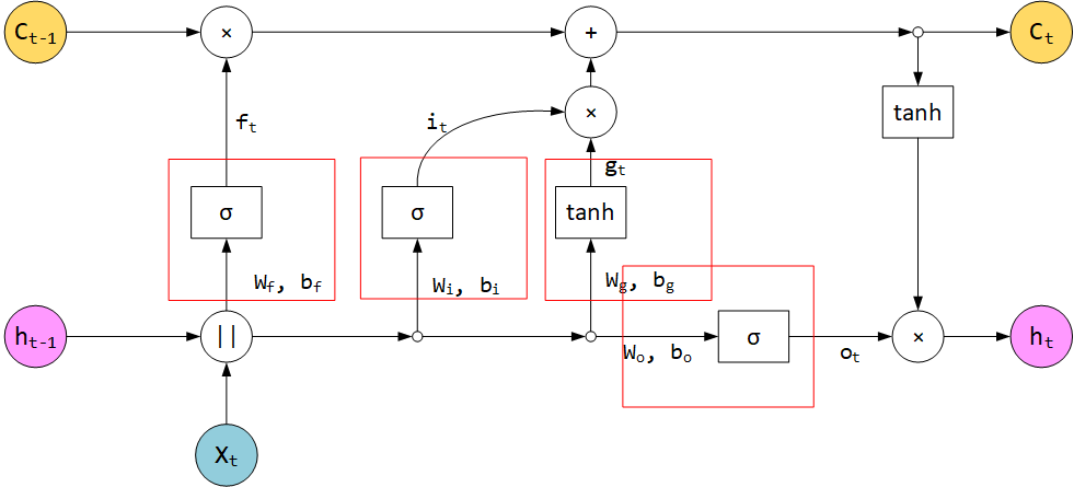
Weighted Connections中基础运算依旧是 y = σ ( W . x + b ) y = \sigma(W.x + b)y =σ(W .x +b )，这里作者避免显式引入非线性激活函数，所以在论文中很多公式没有带激活函数，但是， 如果有激活函数，那么激活值采用激活函数之后的。假设前向计算有 z j = ∑ i z i . ω i j + b j z_j = \sum_i z_i. \omega_{ij} + b_j z j =∑i z i .ωi j +b j ，这里如果引入激活函数，z j z_j z j 就是被激活函数激活后的值，i i i 是 j j j 的前置神经元，LRP针对 j j j 的relevance计算结果为 R j R_j R j ，那么 j → i j \rightarrow i j →i 的relevance 。

R i ← j = z i . ω i j + ϵ . s i g n ( z i ) + δ . b j N z j + ϵ . s i g n ( z j ) . R j R_{i \leftarrow j} = \frac{z_i.\omega_{ij} + \frac{\epsilon . sign(z_i) + \delta.b_j}{N}}{z_j + \epsilon.sign(z_j)}.R_j R i ←j =z j +ϵ.s i g n (z j )z i .ωi j +N ϵ.s i g n (z i )+δ.b j .R j

R i = ∑ j R i ← j R_i = \sum_j R_{i \leftarrow j}R i =j ∑R i ←j

这里作者设置 ϵ = 0.001 , δ = 1.0 , N \epsilon = 0.001, \delta = 1.0, N ϵ=0 .0 0 1 ,δ=1 .0 ,N 是对应神经网络层拥有的神经元数量，s i g n sign s i g n 函数就是非负转1，负转-1的函数。

这里记 R j → R i R_j \rightarrow R_i R j →R i 为 L L LL L L (LRP_Linear)

; 2.2.2.Multiplicative Interactions

Multiplicative Interactions这个概念要和RNN中门的概念结合起来，下面红框框出的是Multiplicative Interactions部分。

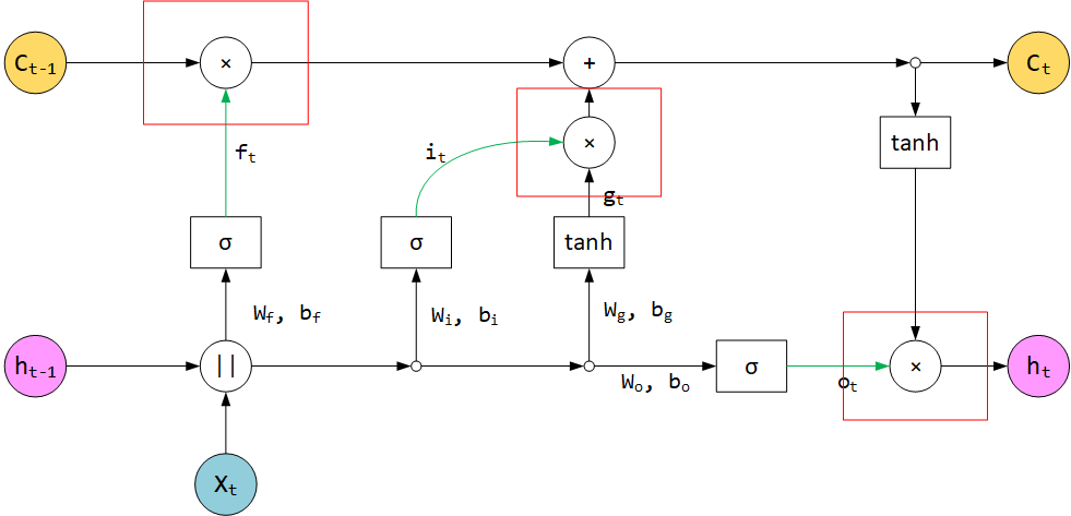
LSTM和GRU中还有一种计算: z j = z g . z s z_j = z_g . z_s z j =z g .z s 。通常称为门，上图红框框出的部分，通常一个操作数值在 [ 0 , 1 ] [0, 1][0 ,1 ] 之间（连接sigmoid），起到一个门的作用，作者称之为 gate neuron z g z_g z g ，另一个称为 source neuron z s z_s z s 。

在C t − 1 × f t C_{t – 1} \times f_t C t −1 ×f t 中，f t f_t f t 为z g z_g z g ，C t − 1 C_{t – 1}C t −1 为z s z_s z s 。
在i t × g t i_t \times g_t i t ×g t 中，i t i_t i t 为z g z_g z g ，g t g_t g t 为z s z_s z s 。
在o t × t a n h ( C t ) o_t \times tanh(C_t)o t ×t a n h (C t ) 中，o t o_t o t 为z g z_g z g ，t a n h ( C t ) tanh(C_t)t a n h (C t ) 为z s z_s z s 。

对于这种情况

R s = R j R_s = R_j R s =R j
R g = 0 R_g = 0 R g =0

等于说在反向运算的时候，绿线标出部分直接清零，计算流图就不包括绿线部分了。Weighted Connections部分只有tanh激活函数参与反向计算。

所以对于上述计算过程可以总结成（无视激活函数，给定 R C t , R h t R_{C_t}, R_{h_t}R C t ,R h t ）：

R C t − 1 = R C t − 1 × f t = L L ( C t − 1 × f t , R C t + R h t ) ∈ R d R_{C_{t – 1}} = R_{C_{t – 1} \times f_t} = LL(C_{t – 1} \times f_t, R_{C_t} + R_{h_t}) \in R^d R C t −1 =R C t −1 ×f t =L L (C t −1 ×f t ,R C t +R h t )∈R d
R g t = R g t × i t = L L ( g t × i t , R C t + R h t ) ∈ R d R_{g_t} = R_{g_t \times i_t} = LL(g_t \times i_t, R_{C_t} + R_{h_t}) \in R^d R g t =R g t ×i t =L L (g t ×i t ,R C t +R h t )∈R d
R h t − 1 = L L ( h t − 1 , R g t ) ∈ R d R_{h_{t – 1}} = LL(h_{t – 1}, R_{g_t}) \in R^d R h t −1 =L L (h t −1 ,R g t )∈R d
R x t = L L ( x t , R g t ) ∈ R d R_{x_t} = LL(x_t, R_{g_t}) \in R^d R x t =L L (x t ,R g t )∈R d

在 R R R 向量初始化上，模型最终输出向量 c = W l e f t . h l e f t T + W r i g h t . h r i g h t T c = W_{left} . h_{left}^T + W_{right}. h_{right}^T c =W l e f t .h l e f t T +W r i g h t .h r i g h t T ，这是个5分类任务，如果目标类别是2，那么 R c = [ 0 , 0 , 1 , 0 , 0 ] R^c = [0, 0, 1, 0, 0]R c =[0 ,0 ,1 ,0 ,0 ] ，其余均初始化0。

2.2.作者代码

LRP函数：

    def lrp(self, w, LRP_class, eps=0.001, bias_factor=0.0):
"""
        Layer-wise Relevance Propagation (LRP) backward pass.

        Compute the hidden layer relevances by performing LRP for the target class LRP_class
        (according to the papers:
            - https://doi.org/10.1371/journal.pone.0130140
            - https://doi.org/10.18653/v1/W17-5221 )
"""

        self.set_input(w)
        self.forward()

        T      = len(self.w)
        d      = int(self.Wxh_Left.shape[0]/4)
        e      = self.E.shape[1]
        C      = self.Why_Left.shape[0]
        idx    = np.hstack((np.arange(0,d), np.arange(2*d,4*d))).astype(int)
        idx_i, idx_g, idx_f, idx_o = np.arange(0,d), np.arange(d,2*d), np.arange(2*d,3*d), np.arange(3*d,4*d)

        Rx       = np.zeros(self.x.shape)
        Rx_rev   = np.zeros(self.x.shape)

        Rh_Left  = np.zeros((T+1, d))
        Rc_Left  = np.zeros((T+1, d))
        Rg_Left  = np.zeros((T,   d))
        Rh_Right = np.zeros((T+1, d))
        Rc_Right = np.zeros((T+1, d))
        Rg_Right = np.zeros((T,   d))

        Rout_mask            = np.zeros((C))
        Rout_mask[LRP_class] = 1.0

        Rh_Left[T-1]  = lrp_linear(self.h_Left[T-1],  self.Why_Left.T , np.zeros((C)), self.s, self.s*Rout_mask, 2*d, eps, bias_factor, debug=False)
        Rh_Right[T-1] = lrp_linear(self.h_Right[T-1], self.Why_Right.T, np.zeros((C)), self.s, self.s*Rout_mask, 2*d, eps, bias_factor, debug=False)

        for t in reversed(range(T)):
            Rc_Left[t]   += Rh_Left[t]
            Rc_Left[t-1]  = lrp_linear(self.gates_Left[t,idx_f]*self.c_Left[t-1],         np.identity(d), np.zeros((d)), self.c_Left[t], Rc_Left[t], 2*d, eps, bias_factor, debug=False)
            Rg_Left[t]    = lrp_linear(self.gates_Left[t,idx_i]*self.gates_Left[t,idx_g], np.identity(d), np.zeros((d)), self.c_Left[t], Rc_Left[t], 2*d, eps, bias_factor, debug=False)
            Rx[t]         = lrp_linear(self.x[t],        self.Wxh_Left[idx_g].T, self.bxh_Left[idx_g]+self.bhh_Left[idx_g], self.gates_pre_Left[t,idx_g], Rg_Left[t], d+e, eps, bias_factor, debug=False)
            Rh_Left[t-1]  = lrp_linear(self.h_Left[t-1], self.Whh_Left[idx_g].T, self.bxh_Left[idx_g]+self.bhh_Left[idx_g], self.gates_pre_Left[t,idx_g], Rg_Left[t], d+e, eps, bias_factor, debug=False)

            Rc_Right[t]  += Rh_Right[t]
            Rc_Right[t-1] = lrp_linear(self.gates_Right[t,idx_f]*self.c_Right[t-1],         np.identity(d), np.zeros((d)), self.c_Right[t], Rc_Right[t], 2*d, eps, bias_factor, debug=False)
            Rg_Right[t]   = lrp_linear(self.gates_Right[t,idx_i]*self.gates_Right[t,idx_g], np.identity(d), np.zeros((d)), self.c_Right[t], Rc_Right[t], 2*d, eps, bias_factor, debug=False)
            Rx_rev[t]     = lrp_linear(self.x_rev[t],     self.Wxh_Right[idx_g].T, self.bxh_Right[idx_g]+self.bhh_Right[idx_g], self.gates_pre_Right[t,idx_g], Rg_Right[t], d+e, eps, bias_factor, debug=False)
            Rh_Right[t-1] = lrp_linear(self.h_Right[t-1], self.Whh_Right[idx_g].T, self.bxh_Right[idx_g]+self.bhh_Right[idx_g], self.gates_pre_Right[t,idx_g], Rg_Right[t], d+e, eps, bias_factor, debug=False)

        return Rx, Rx_rev[::-1,:], Rh_Left[-1].sum()+Rc_Left[-1].sum()+Rh_Right[-1].sum()+Rc_Right[-1].sum()

lrp_linear函数

def lrp_linear(hin, w, b, hout, Rout, bias_nb_units, eps, bias_factor=0.0, debug=False):
"""
    LRP for a linear layer with input dim D and output dim M.

    Args:
    - hin: forward pass input, of shape (D,)
    - w: connection weights, of shape (D, M)
    - b: biases, of shape (M,)
    - hout: forward pass output, of shape (M,) (unequal to np.dot(w.T,hin)+b if more than one incoming layer!)
    - Rout:           relevance at layer output, of shape (M,)
    - bias_nb_units:  total number of connected lower-layer units (onto which the bias/stabilizer contribution is redistributed for sanity check)
    - eps:            stabilizer (small positive number)
    - bias_factor:    set to 1.0 to check global relevance conservation, otherwise use 0.0 to ignore bias/stabilizer redistribution (recommended)
    Returns:
    - Rin:            relevance at layer input, of shape (D,)
"""
    sign_out = np.where(hout[na,:]>=0, 1., -1.)
    numer = (w * hin[:,na]) + ( bias_factor * (b[na,:]*1. + eps*sign_out*1.) / bias_nb_units )

    denom = hout[na,:] + (eps*sign_out*1.)
    message = (numer/denom) * Rout[na,:]
    Rin = message.sum(axis=1)
    if debug:
        print("local diff: ", Rout.sum() - Rin.sum())

    return Rin

lrp_linear针对神经网络中每一个线性操作 y = W . x + b y = W.x + b y =W .x +b，给定 y y y 处relevance R y R_y R y ，计算 x x x 处值 R x R_x R x ， numer对应 z i . ω i j + ϵ . s i g n ( z i ) + δ . b j N z_i.\omega_{ij} + \frac{\epsilon . sign(z_i) + \delta.b_j}{N}z i .ωi j +N ϵ.s i g n (z i )+δ.b j ， denom对应 z j + ϵ . s i g n ( z j ) z_j + \epsilon.sign(z_j)z j +ϵ.s i g n (z j )。

回到 LRP函数，针对 C t , h t = L S T M C e l l ( C t − 1 , h t − 1 , x t ) C_t, h_t = LSTMCell(C_{t – 1}, h_{t – 1}, x_t)C t ,h t =L S T M C e l l (C t −1 ,h t −1 ,x t ),，给定 C t C_t C t 的relevance值 R C t R_{C_t}R C t 和 h t h_t h t 的relevance值 R h t R_{h_t}R h t ，需要计算 R x t , R h t − 1 , R C t − 1 R_{x_t}, R_{h_{t – 1}}, R_{C_{t – 1}}R x t ,R h t −1 ,R C t −1 。相应计算如下：

Rc_Left[t]   += Rh_Left[t]
Rc_Left[t-1]  = lrp_linear(self.gates_Left[t,idx_f]*self.c_Left[t-1],         np.identity(d), np.zeros((d)), self.c_Left[t], Rc_Left[t], 2*d, eps, bias_factor, debug=False)
Rg_Left[t]    = lrp_linear(self.gates_Left[t,idx_i]*self.gates_Left[t,idx_g], np.identity(d), np.zeros((d)), self.c_Left[t], Rc_Left[t], 2*d, eps, bias_factor, debug=False)
Rx[t]         = lrp_linear(self.x[t],        self.Wxh_Left[idx_g].T, self.bxh_Left[idx_g]+self.bhh_Left[idx_g], self.gates_pre_Left[t,idx_g], Rg_Left[t], d+e, eps, bias_factor, debug=False)
Rh_Left[t-1]  = lrp_linear(self.h_Left[t-1], self.Whh_Left[idx_g].T, self.bxh_Left[idx_g]+self.bhh_Left[idx_g], self.gates_pre_Left[t,idx_g], Rg_Left[t], d+e, eps, bias_factor, debug=False)

再给一个LSTM图

红色线条表示 R C t − 1 R_{C_{t – 1}}R C t −1 和 R g t R_{g_t}R g t 的计算流程，绿色线条表示 R x t R_{x_t}R x t 和 R h t − 1 R_{h_{t – 1}}R h t −1 的计算流程。

三.扩展到GRU

3.1.GRU

流程如下：

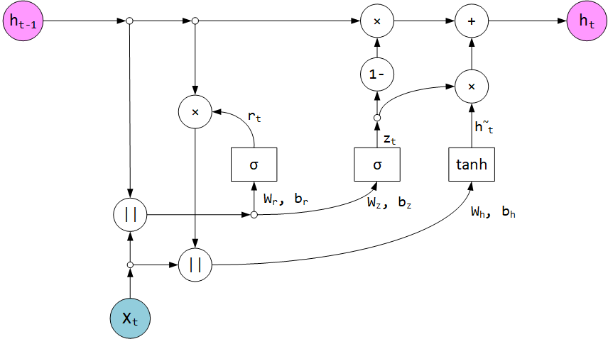
涉及到的输入和模型参数：

x t ∈ R e x_t \in R^e x t ∈R e
h t ∈ R d h_t \in R^d h t ∈R d
W r , W z , W h ∈ R ( d + e ) × d W_r, W_z, W_h \in R^{(d + e) \times d}W r ,W z ,W h ∈R (d +e )×d
b r , b z , b h ∈ R d b_r, b_z, b_h \in R^d b r ,b z ,b h ∈R d
r t , z t , h ~ t ∈ R d r_t, z_t, \widetilde h_t \in R^d r t ,z t ,h t ∈R d

计算过程：

r t = σ ( W r . [ h t − 1 ; x t ] + b r ) r_t = \sigma(W_r.[h_{t – 1}; x_t] + b_r)r t =σ(W r .[h t −1 ;x t ]+b r )
z t = σ ( W z . [ h t − 1 ; x t ] + b z ) z_t = \sigma(W_z.[h_{t – 1}; x_t] + b_z)z t =σ(W z .[h t −1 ;x t ]+b z )
h ~ t = t a n h ( W h . [ r t × h t − 1 ; x t ] + b h ) \widetilde h_t = tanh(W_h.[r_t \times h_{t-1}; x_t] + b_h)h t =t a n h (W h .[r t ×h t −1 ;x t ]+b h )
h t = ( 1 − z t ) × h t − 1 + z t × h ~ t h_t = (1 – z_t) \times h_{t – 1} + z_t \times \widetilde h_t h t =(1 −z t )×h t −1 +z t ×h t

; 3.2.GRU的Relevance计算部分

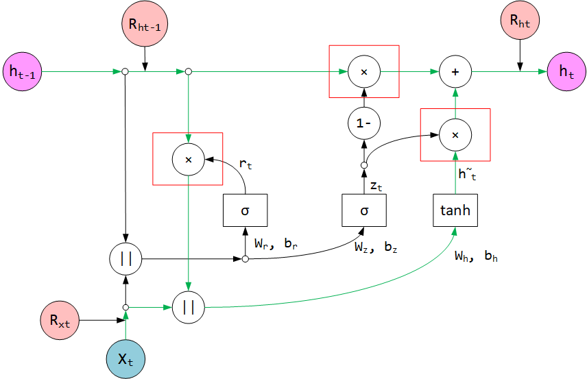
按照前面的理论，R x t R_{x_t}R x t 和 R h t − 1 R_{h_{t-1}}R h t −1 的计算过程按绿线所示反向进行，因为红框乘法部分 z g z_g z g 会被忽略掉，所以指挥按一个流程进行。

四.参考文献

[1] Arras, L. , et al. “Explaining Recurrent Neural Network
Predictions in Sentiment Analysis.” EMNLP’17 Workshop on Computational
Approaches to Subjectivity, Sentiment & Social Media Analysis 2017.

Original: https://blog.csdn.net/qq_44370676/article/details/121490050
Author: I still …
Title: 可解释性研究 -LRP-for-LSTM

原创文章受到原创版权保护。转载请注明出处：https://www.johngo689.com/710550/

转载文章受原作者版权保护。转载请注明原作者出处！

人工智能

【自取】最近整理的，有需要可以领取学习：

Linux核心资料大放送~

全栈面试题汇总（持续更新&可下载）

一个提高学习100%效率的工具！

【超详细】深度学习面试题目！

LeetCode Python刷题答案下载！

LeetCode Java版刷题答案下载！

LeetCode C++ 版本，抓紧保存！

LeetCode GO语言刷题答案下载！

OpenCV-Python:简单实现人脸识别

安装 pip install numpy pip install opencv-python pip install opencv-contrib-python OpenCV主要模…

人工智能 2023年7月18日
0084
UnicodeDecodeError: ‘utf-8‘ codec can‘t decode byte 0xff in position 41: invalid start byte

在代码再现过程中，笔者在读取数据时遇到错误： [En] In the process of code reproduction, the author encountered an…

人工智能 2023年5月27日
0085
【R语言】实验四数据分析

hospital-data 数据集数据是关于一些医院的基础信息，数据包含13个字段，包含的字段分别为：供应商编号、医院名、地址 1、地址2、地址3、所处城市、所处州、邮编、所处乡…

人工智能 2023年6月11日
0076
单层感知器线性分类、多层感知器非线性分类样例调用matlab神经网络工具箱实现

%给定样本输入向量P，目标输出向量T %net = newp（PR,S,TF,LF） %PR为输入矢量的取值范围的最大值和最小值 S为神经元的个数 TF为网络的传递函数默认为ha…

人工智能 2023年7月3日
0063
强化学习——PyTorch 实现 Advantage Actor-Critic (A2C)

前言本博客的理论知识来自王树森老师《深度强化学习》，这本书写得简直太好了，强烈推荐，只是现在还在校对没出版，可能有些小瑕疵，但并不影响阅读和学习。 Advantage Actor…

人工智能 2023年7月22日
0045
Collaborative算法如何处理用户的评分偏好或偏差

问题描述 Collaborative filtering（协同过滤）算法是一种常用于推荐系统中的算法，通过分析用户的历史行为数据，如评分、购买记录等，来预测用户对未知产品的喜好程度…

人工智能 2024年1月4日
0037
Spark RDD转换为DataFrame

bash;gutter:true;</p> <h1>构造case class，利用反射机制隐式转换</h1> <p>scala&gt…

人工智能 2023年6月2日
0088
Python–DataFrame分组-GroupBy

DataFame分组功能及其他配合使用方法分组统计 👉 GroupBy *.groupby(by=None,axis=0,level=None,as_index=True,sor…

人工智能 2023年6月2日
00100
物联网应用系统设计复习提纲-上

目录 1.掌握Linux常用的基本命令功能、语法结构、用法等。 2.什么是操作系统OS？ 3.现代操作系统类型【五大类】 (1)分时系统 (2)实时操作系统 (3)微机操作系统 (…

人工智能 2023年6月29日
00111
Pandas-DataFrame使用

文章目录 * – 1.创建DataFrame数据 – + 1.1 给DataFrame添加数据 + 1.3 给行索引和列索引起名 + 1.4 判断数据是否在…

人工智能 2023年7月8日
0054
【笔记】PyTorch快速入门：简单的神经网络模型

神经网络神经网络是一些层或者模块，对数据进行处理。 torch.nn提供了诸多构造神经网络的模块，模块化的结构方便了管理复杂结构。接下来以在FashionMNIST上构造一个图…

人工智能 2023年6月4日
00118
【实验技术笔记】细胞表型检测之细胞增殖（CCK-8法 + BrdU掺入法 + 平板克隆）

文章目录 1. 细胞增殖的定义 2. 检测细胞数量：CCK-8 法 3. 检测细胞增殖：BrdU 掺入法 4. 检测细胞增殖：平板克隆细胞增殖的定义通过检测细胞数量来判断细胞…

人工智能 2023年7月28日
0083
PaddleDetection快速上手及问题排查

1. PaddlePaddle环境安装 1.1 目前飞桨支持的环境查看 1.2 CPU版本安装注1，import paddle后报错 2. 安装PaddleDetection 2…

人工智能 2023年7月12日
0096
matlab神经网络报错net.LW{1,1}must be a 7-by-5 matrix解决方法

笔者是在使用GA、PSO等算法优化bp网络权值时出现的这个问题。我是85的网络，你为啥向我要75的矩阵啊55555 T^T 报错位置出现在网络pso的个体（维度为权值+阈值）赋给…

人工智能 2023年7月14日
0036
python+html实现前后端数据交互界面显示

最近刚刚开始学习如何将python后台与html前端结合起来，现在写一篇blog记录一下，我采用的是前后端不分离形式。话不多说，先来实现一个简单的计算功能吧，前端输入计算的数据，…

人工智能 2023年7月4日
0058
[ 网络安全基础篇 ]常见 Web 漏洞的描述及其修复建议（相对全面）

抵扣说明： 1.余额是钱包充值的虚拟货币，按照1:1的比例进行支付金额的抵扣。2.余额无法直接购买下载，可以购买VIP、C币套餐、付费专栏及课程。 Original: https:…

人工智能 2023年6月2日
0074

2024 年 4 月
一	二	三	四	五	六	日
1	2	3	4	5	6	7
8	9	10	11	12	13	14
15	16	17	18	19	20	21
22	23	24	25	26	27	28
29	30