

步骤
写在前面——按照生信技能树的学习路线,学完R语言就该学习GEO数据挖掘了。有人说GEO数据挖掘可以快速发文(https://zhuanlan.zhihu.com/p/36303146),不知道靠不靠谱。反正学一学总没有坏处。看完Jimmy老师的视频,写一篇总结方便日后复习。这里有很多操作在
《生信人的20个R语言习题》
都可以见到,那里写的更加详细。
视频教程:https://www.bilibili.com/video/BV1is411H7Hq?p=1
代码地址:https://github.com/jmzeng1314/GEO
STEP1:表达矩阵ID转换
首先理解下面的4个概念:
GEO Platform (GPL)
GEO Sample (GSM)
GEO Series (GSE)
GEO Dataset (GDS)
理解起来也很容易。一篇文章可以有一个或者多个GSE数据集,一个GSE里面可以有一个或者多个GSM样本。多个研究的GSM样本可以根据研究目的整合为一个GDS,不过GDS本身用的很少。而每个数据集都有着自己对应的芯片平台,就是GPL。
用R获取芯片探针与基因的对应关系三部曲-bioconductor
http://www.bio-info-trainee.com/1399.html
if(F){
  suppressPackageStartupMessages(library(GEOquery))
  gset  getGEO('GSE42872', destdir=".",
                 AnnotGPL = F,
                 getGPL = F)
  save(gset,file='GSE42872_gset.Rdata')
}
load('GSE42872_gset.Rdata')

exprSet  exprs(gset[[1]])
pdata  pData(gset[[1]])
group_list  c(rep('control', 3), rep('case', 3))

suppressPackageStartupMessages(library(hugene10sttranscriptcluster.db))

ls("package:hugene10sttranscriptcluster.db")
ids  toTable(hugene10sttranscriptclusterSYMBOL)

table(rownames(exprSet) %in% ids$probe_id)
dim(exprSet)
exprSet  exprSet[(rownames(exprSet) %in% ids$probe_id),]
dim(exprSet)

ids  ids[match(rownames(exprSet),ids$probe_id),]
dim(ids)

tmp  by(exprSet,ids$symbol,
          function(x) rownames(x)[which.max(rowMeans(x))])
tmp[1:20]
probes  as.character(tmp)
exprSet  exprSet[rownames(exprSet) %in% probes, ]
dim(exprSet)
dim(ids)

rownames(exprSet)  ids[match(rownames(exprSet),ids$probe_id),2]

save(exprSet, group_list, file = 'GSE42872_new_exprSet.Rdata')
转换前的exprSet


转换后的exprSet

STEP2:差异分析
load('GSE42872_new_exprSet.Rdata')

library(reshape2)
m_exprSet  melt(exprSet)
head(m_exprSet)
colnames(m_exprSet)  c("symbol", "sample", "value")
head(m_exprSet)
m_exprSet$group  rep(group_list, each = nrow(exprSet))
head(m_exprSet)

library(ggplot2)
ggplot(m_exprSet, aes(x = sample, y = value, fill = group)) + geom_boxplot()

colnames(exprSet)  paste(group_list,1:6,sep='')
hc  hclust(dist(t(exprSet)))
nodePar  list(lab.cex = 0.6, pch = c(NA, 19), cex = 0.7, col = "blue")
par(mar=c(5,5,5,10))
plot(as.dendrogram(hc), nodePar = nodePar,  horiz = TRUE)

library(limma)

design  model.matrix(~0 + factor(group_list))
colnames(design)  levels(factor(group_list))
rownames(design)  colnames(exprSet)
design

contrast.matrix  makeContrasts("case-control" ,levels = design)

contrast.matrix

fit  lmFit(exprSet,design)

fit2  contrasts.fit(fit, contrast.matrix)

fit2  eBayes(fit2)

tempOutput  topTable(fit2, coef=1, n=Inf)

nrDEG  na.omit(tempOutput)

head(nrDEG)

DEG  nrDEG

logFC_cutoff  with(DEG, mean(abs(logFC)) + 2*sd(abs(logFC)))

DEG$result  as.factor(ifelse(DEG$P.Value < 0.05 & abs(DEG$logFC) > logFC_cutoff,
                               ifelse(DEG$logFC >logFC_cutoff, 'UP', 'DOWN'), 'NOT')

)

this_tile  paste0('Cutoff for logFC is', round(logFC_cutoff, 3),
                    '\nThe number of UP gene is ', nrow(DEG[DEG$result == 'UP', ]),
                    '\nThe number of DOWN gene is ', nrow(DEG[DEG$result == 'DOWN', ]))
this_tile

head(DEG)

library(ggplot2)

ggplot(data=DEG, aes(x=logFC, y=-log10(P.Value), color=result)) +
  geom_point(alpha=0.4, size=1.75) +
  theme_set(theme_set(theme_bw(base_size=20)))+
  xlab("log2 fold change") + ylab("-log10 p-value") +
  ggtitle( this_tile ) + theme(plot.title = element_text(size=15,hjust = 0.5))+
  scale_colour_manual(values = c('blue','black','red'))

save(exprSet, group_list, nrDEG, DEG, file = 'GSE42872_DEG.Rdata')
?topTable :Value
DEG中的行变量对应的说明
A dataframe with a row for the number top genes and the following columns:
genelist:one or more columns of probe annotation, if genelist was included as input
logFC:estimate of the log2-fold-change corresponding to the effect or contrast (for topTableF there may be several columns of log-fold-changes)
CI.L:left limit of confidence interval for logFC (if confint=TRUE or confint is numeric)
CI.R:right limit of confidence interval for logFC (if confint=TRUE or confint is numeric)
AveExpr:average log2-expression for the probe over all arrays and channels, same as Amean in the MarrayLM object
t:moderated t-statistic (omitted for topTableF)
F:moderated F-statistic (omitted for topTable unless more than one coef is specified)
P.Value:raw p-value
adj.P.Value:adjusted p-value or q-value
B:log-odds that the gene is differentially expressed (omitted for topTreat)


STEP3:KEGG数据库注释
生信技能树:差异分析得到的结果注释一文就够
差异分析通过自定义的阈值挑选了有统计学显著的基因列表,我们需要对它们进行注释才能了解其功能,最常见的就是GO/KEGG数据库注释,当然也可以使用Reactome和Msigdb数据库来进行注释。最常见的注释方法就是超几何分布检验。
load('GSE42872_DEG.Rdata')
suppressPackageStartupMessages(library(clusterProfiler))
suppressPackageStartupMessages(library(org.Hs.eg.db))
gene head(rownames(nrDEG), 1000)
gene.df bitr(gene, fromType = "SYMBOL",
toType = c("ENSEMBL", "ENTREZID"),
OrgDb = org.Hs.eg.db)
head(gene.df)
kk enrichKEGG(gene = gene.df$ENTREZID, organism = "hsa",
pvalueCutoff = 0.05)
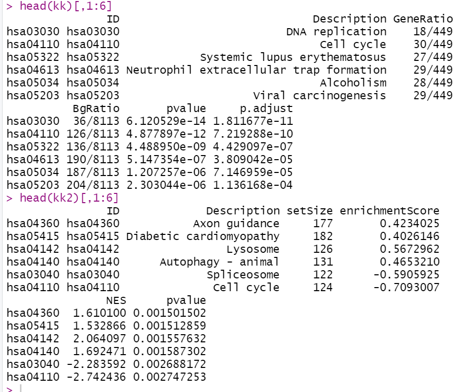
head(kk)[,1:6]
data(geneList, package = "DOSE")
boxplot(geneList)
head(geneList)
boxplot(nrDEG$logFC)
geneList nrDEG$logFC
names(geneList) rownames(nrDEG)
head(geneList)
gene.symbol bitr(names(geneList), fromType = "SYMBOL",
toType = c("ENSEMBL", "ENTREZID"),
OrgDb = org.Hs.eg.db)
head(gene.symbol)
tmp data.frame(SYMBOL = names(geneList),
logFC = as.numeric(geneList))
tmp merge(tmp, gene.symbol, by = 'SYMBOL')
geneList tmp$logFC
names(geneList) tmp$ENTREZID
head(geneList)
geneList sort(geneList, decreasing = T)
kk2 gseKEGG(geneList = geneList,
organism = 'hsa',
nPerm = 1000,
minGSSize = 120,
pvalueCutoff = 0.05,
verbose = FALSE)
head(kk2)[,1:6]
gseaplot(kk2, geneSetID = "hsa04142")

完整代码
setwd(dir = "geo_learn/")

if(F){
  suppressPackageStartupMessages(library(GEOquery))
  gset  getGEO('GSE42872', destdir=".",
                 AnnotGPL = F,
                 getGPL = F)
  save(gset,file='GSE42872_gset.Rdata')
}
load('GSE42872_gset.Rdata')

exprSet  exprs(gset[[1]])
pdata  pData(gset[[1]])
group_list  c(rep('control', 3), rep('case', 3))

suppressPackageStartupMessages(library(hugene10sttranscriptcluster.db))

ids  toTable(hugene10sttranscriptclusterSYMBOL)

table(rownames(exprSet) %in% ids$probe_id)

exprSet  exprSet[(rownames(exprSet) %in% ids$probe_id),]

ids  ids[match(rownames(exprSet),ids$probe_id),]

tmp  by(exprSet,ids$symbol,
          function(x) rownames(x)[which.max(rowMeans(x))])

probes  as.character(tmp)
exprSet  exprSet[rownames(exprSet) %in% probes, ]

rownames(exprSet)  ids[match(rownames(exprSet),ids$probe_id),2]

save(exprSet, group_list, file = 'GSE42872_new_exprSet.Rdata')

load('GSE42872_new_exprSet.Rdata')

library(reshape2)
m_exprSet  melt(exprSet)
head(m_exprSet)
colnames(m_exprSet)  c("symbol", "sample", "value")
head(m_exprSet)
m_exprSet$group  rep(group_list, each = nrow(exprSet))
head(m_exprSet)

library(ggplot2)
ggplot(m_exprSet, aes(x = sample, y = value, fill = group)) + geom_boxplot()

colnames(exprSet)  paste(group_list,1:6,sep='')
hc  hclust(dist(t(exprSet)))
nodePar  list(lab.cex = 0.6, pch = c(NA, 19), cex = 0.7, col = "blue")
par(mar=c(5,5,5,10))
plot(as.dendrogram(hc), nodePar = nodePar,  horiz = TRUE)

library(limma)
design  model.matrix(~0 + factor(group_list))
colnames(design)  levels(factor(group_list))
rownames(design)  colnames(exprSet)
design

contrast.matrix  makeContrasts("case-control" ,levels = design)

contrast.matrix

fit  lmFit(exprSet,design)

fit2  contrasts.fit(fit, contrast.matrix)

fit2  eBayes(fit2)

tempOutput  topTable(fit2, coef=1, n=Inf)
nrDEG  na.omit(tempOutput)
head(nrDEG)

DEG  nrDEG
logFC_cutoff  with(DEG, mean(abs(logFC)) + 2*sd(abs(logFC)))
DEG$result  as.factor(ifelse(DEG$P.Value < 0.05 & abs(DEG$logFC) > logFC_cutoff,
                               ifelse(DEG$logFC >logFC_cutoff, 'UP', 'DOWN'), 'NOT')

)

this_tile  paste0('Cutoff for logFC is', round(logFC_cutoff, 3),
                    '\nThe number of UP gene is ', nrow(DEG[DEG$result == 'UP', ]),
                    '\nThe number of DOWN gene is ', nrow(DEG[DEG$result == 'DOWN', ]))
this_tile

head(DEG)
library(ggplot2)
ggplot(data=DEG, aes(x=logFC, y=-log10(P.Value), color=result)) +
  geom_point(alpha=0.4, size=1.75) +
  theme_set(theme_set(theme_bw(base_size=20)))+
  xlab("log2 fold change") + ylab("-log10 p-value") +
  ggtitle( this_tile ) + theme(plot.title = element_text(size=15,hjust = 0.5))+
  scale_colour_manual(values = c('blue','black','red'))

save(exprSet, group_list, nrDEG, DEG, file = 'GSE42872_DEG.Rdata')

load('GSE42872_DEG.Rdata')
suppressPackageStartupMessages(library(clusterProfiler))
suppressPackageStartupMessages(library(org.Hs.eg.db))

gene  head(rownames(nrDEG), 1000)

gene.df  bitr(gene, fromType = "SYMBOL",
                toType = c("ENSEMBL", "ENTREZID"),
                OrgDb = org.Hs.eg.db)
head(gene.df)

kk  enrichKEGG(gene = gene.df$ENTREZID, organism = "hsa",
                 pvalueCutoff = 0.05)
head(kk)[,1:6]

data(geneList, package = "DOSE")
boxplot(geneList)
head(geneList)

boxplot(nrDEG$logFC)
geneList  nrDEG$logFC
names(geneList)  rownames(nrDEG)
head(geneList)

gene.symbol  bitr(names(geneList), fromType = "SYMBOL",
                toType = c("ENSEMBL", "ENTREZID"),
                OrgDb = org.Hs.eg.db)
head(gene.symbol)

tmp  data.frame(SYMBOL = names(geneList),
                  logFC = as.numeric(geneList))
tmp  merge(tmp, gene.symbol, by = 'SYMBOL')
geneList  tmp$logFC
names(geneList)  tmp$ENTREZID
head(geneList)

geneList  sort(geneList, decreasing = T)

kk2  gseKEGG(geneList     = geneList,
               organism     = 'hsa',
               nPerm        = 1000,
               minGSSize    = 120,
               pvalueCutoff = 0.05,
               verbose      = FALSE)
head(kk2)[,1:6]

gseaplot(kk2, geneSetID = "hsa04142")
Original: https://blog.csdn.net/narutodzx/article/details/121950483
Author: Dzfly..
Title: 生信学习——GEO数据挖掘
原创文章受到原创版权保护。转载请注明出处:https://www.johngo689.com/696993/
转载文章受原作者版权保护。转载请注明原作者出处!