

回归综合案例——利用回归模型预测鲍鱼年龄
1 数据集探索性分析
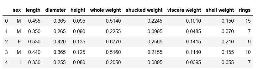
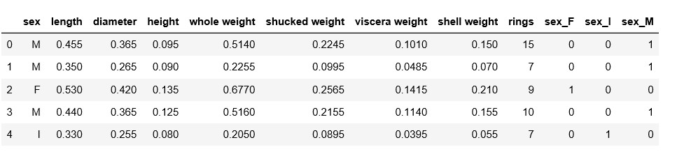
首先将鲍鱼数据集abalone_dataset.csv读取为pandas的DataFrame格式。
import pandas as pd
import warnings
warnings.filterwarnings('ignore')
data = pd.read_csv(r"C:\Users\86182\Desktop\abalone_dataset.csv")
data.head()

data.shape
(4177,9)
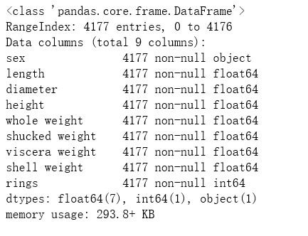
data.info()
data.describe()
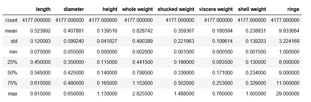
数据集一共有4177个样本,每个样本有9个特征,其中rings为鲍鱼环数,能够代表鲍鱼年龄,是预测变量。除了sex为离散特征,其余都为连续变量。
观察sex列的取值分布情况。
import seaborn as sns
import matplotlib.pyplot as plt
%matplotlib inline
sns.countplot(x = "sex",data = data)
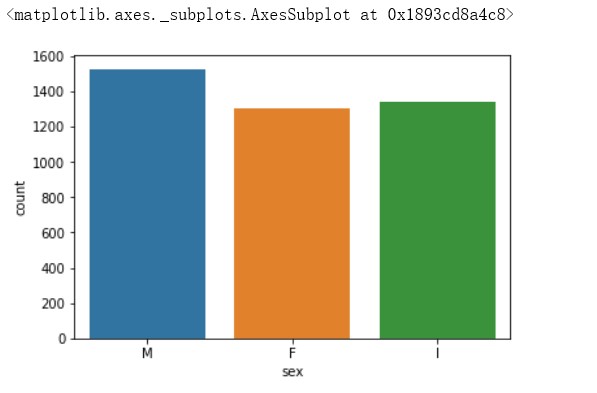
data['sex'].value_counts()

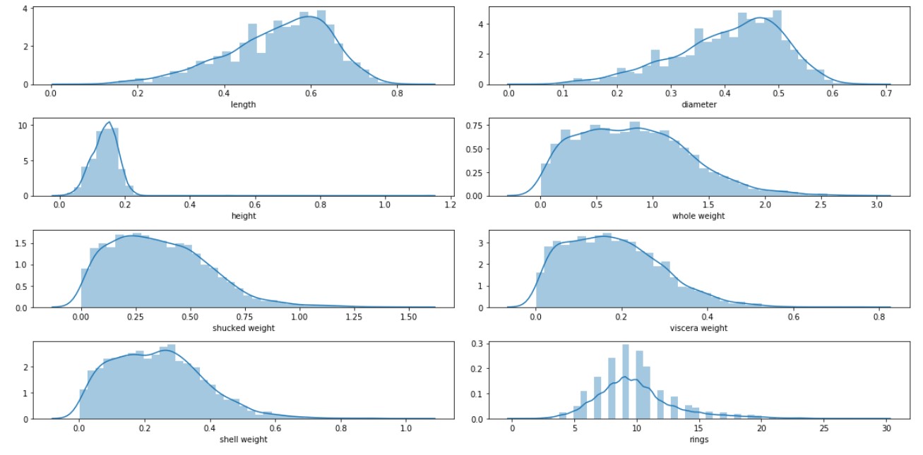
对于连续特征,可以使用seaborn的distplot函数绘制直方图观察特征取值情况。我们将8个连续特征的直方图绘制在一个4行2列的子图布局中。
i = 1
plt.figure(figsize=(16,8))
for col in data.columns[1:]:
    plt.subplot(4,2,i)
    i = i + 1
    sns.distplot(data[col])
    plt.tight_layout()
sns.pairplot(data,hue="sex")
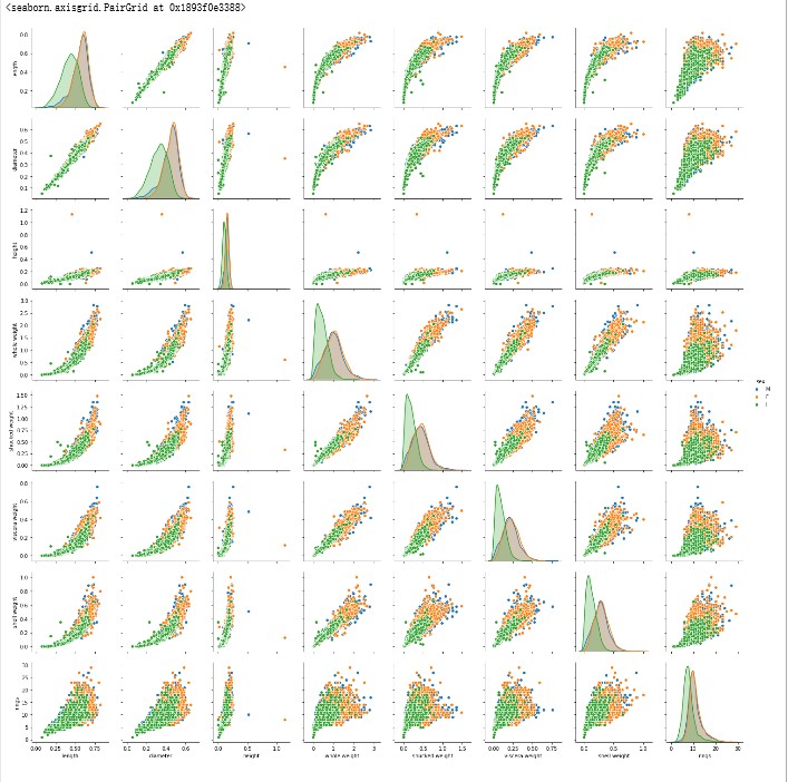
从以上连续特征之间的散点图我们可以看到一些基本的结果:
●例如从第一行可以看到鲍鱼的长度length 和鲍鱼直径diameter 、鲍鱼高度height 存在明显的线性关系。鲍鱼长度与鮑鱼的四种重量之间存在明显的非线性关系。
●观察最后一行,鲍鱼环数rings 与各个特征均存在正相关性,中与height 的线性关系最为直观。
●观察对角线上的直方图,可以看到幼鲍鱼( sex 取值为”)在各个特征上的取值明显小于其他成年鲍鱼。而雄性鲍鱼( sex取值为”M”)和雌性鲍鱼( sex 取值为”F”)各个特征取值分布没有明显的差异。
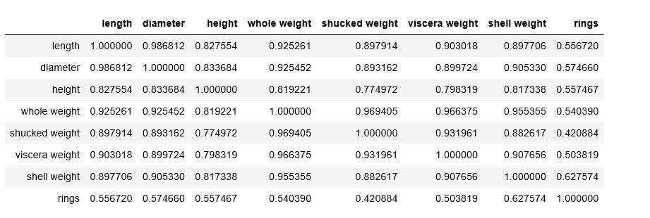
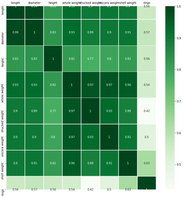
为了定量地分析特征之间的线性相关性,我们计算特征之间的相关系数矩阵,并借助热力图将相关性可视化。
corr_df = data.corr()
corr_df
fig,ax = plt.subplots(figsize=(12,12))

ax = sns.heatmap(corr_df,linewidths=.5,
                cmap="Greens",
                annot=True,
                xticklabels=corr_df.columns,
                yticklabels=corr_df.index)
ax.xaxis.set_label_position('top')
ax.xaxis.tick_top()
2 鲍鱼数据预处理
2.1 对sex特征进行Onehot编码,便于后续模型纳入哑变量
使用pandas的get_dummies函数对sex特征做Onehot编码处理。
sex_onehot = pd.get_dummies(data["sex"],prefix="sex")
data[sex_onehot.columns] = sex_onehot
data.head()
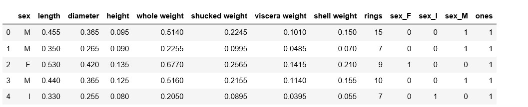
2.2 添加取值为 1 的特征
data["ones"] = 1
data.head()
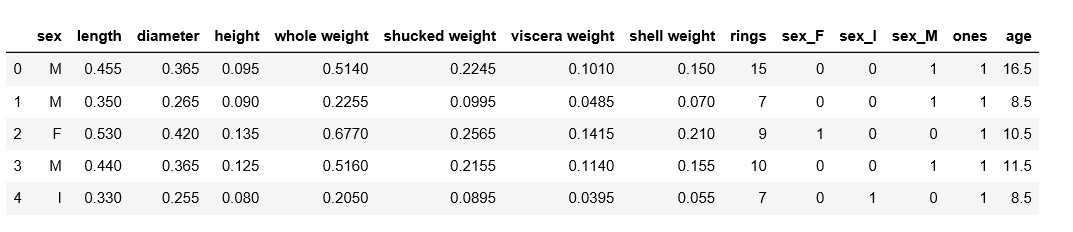
2.3 根据鲍鱼环计算年龄
一般每过一年,鲍鱼就会在壳上留下一道深深地印记,这叫生长纹,就相当于树木的年轮。在本数据集中,我们要预测的是鲍鱼的年龄,可以通过环数rings加上1.5得到。
data["age"] = data["rings"] + 1.5
data.head()
2.4 筛选特征
将预测目标设置为age列,然后构造两组特征,一组包含ones,一组包含ones。对于sex相关的列,我们只使用sex_F和sex_M。
y = data["age"]
features_with_ones = ["length","diameter","height","whole weight","shucked weight",
                      "viscera weight","shell weight","sex_F","sex_M","ones"]
features_without_ones = ["length","diameter","height","whole weight","shucked weight",
                      "viscera weight","shell weight","sex_F","sex_M"]
X = data[features_with_ones]
data.columns

2.5 将鲍鱼数据集划分为训练集和测试集
将数据集随机划分为训练集和测试集,其中80%样本为训练集,剩余20%样本为测试集。
from sklearn.model_selection import train_test_split
X_train,X_test,y_train,y_test = train_test_split(X,y,test_size=0.2,random_state=111)
3 实现线性回归和岭回归
3.1 使用Numpy实现线性回归
如果矩阵xTx为满秩(行列式不为0),则简单线性回归的解为W=(XTx)-1xTy。实现一个函数linear _regression, 其输入为训练集特征部分和标签部分,返回回归系数向量。我们借助numpy 工具中的np. linalg. det函数和np. linalg. inv函数分别求矩阵的行列式和矩阵的逆。
import numpy as np
def linear_regression(X,y):
    w = np.zeros_like(X.shape[1])
    if np.linalg.det(X.T.dot(X)) != 0:
        w = np.linalg.inv(X.T.dot(X)).dot(X.T).dot(y)
    return w
使用上述实现的线性回归模型在鲍鱼训练集上训练模型。
w1 = linear_regression(X_train,y_train)
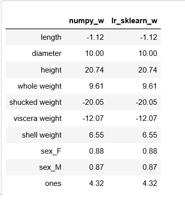
w1 = pd.DataFrame(data = w1,index=X.columns,columns = ["numpy_w"])
w1.round(decimals=2)

可见我们求得的模型为:
y=-l.12 х length + 10 х diameter + 20.74 х height + 9.61 х whole_ weight-20.05 х shucked_ weight – 12.07 х viscera_ weight + 6.55 х shell_ weight + 0.88x sex_ F+0.87 x sex_ M + 4.32
3.2 使用sklearn实现线性回归
from sklearn.linear_model import LinearRegression
lr = LinearRegression()
lr.fit(X_train[features_without_ones],y_train)
print(lr.coef_)

w_lr = []
w_lr.extend(lr.coef_)
w_lr.append(lr.intercept_)
w1["lr_sklearn_w"] = w_lr
w1.round(decimals=2)
3.3 使用Numpy实现岭回归(Ridge)
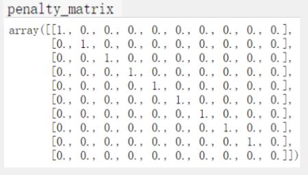
def ridge_regression(X,y,ridge_lambda):
    penalty_matrix = np.eye(X.shape[1])
    penalty_matrix[X.shape[1] - 1][X.shape[1] - 1] = 0
    w = np.linalg.inv(X.T.dot(X) + ridge_lambda * penalty_matrix).dot(X.T).dot(y)
    return w
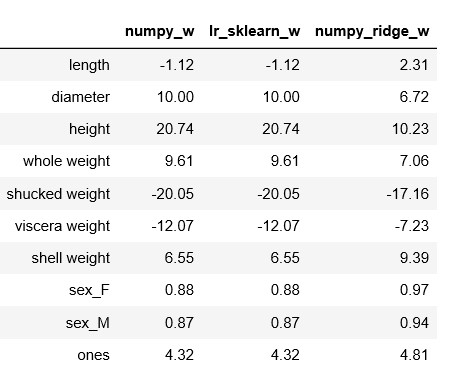
在鲍鱼训练集上使用ridge_regression函数训练岭回归模型,正则化系数设置为1.
w2 = ridge_regression(X_train,y_train,1.0)
print(w2)

w1["numpy_ridge_w"] = w2
w1.round(decimals=2)
3.4 利用sklearn实现岭回归
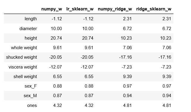
与sklearn中岭回归对比,同样正则化系数设置为1。
from sklearn.linear_model import Ridge
ridge = Ridge(alpha=1.0)
ridge.fit(X_train[features_without_ones],y_train)
w_ridge = []
w_ridge.extend(ridge.coef_)
w_ridge.append(ridge.intercept_)
w1["ridge_sklearn_w"] = w_ridge
w1.round(decimals=2)
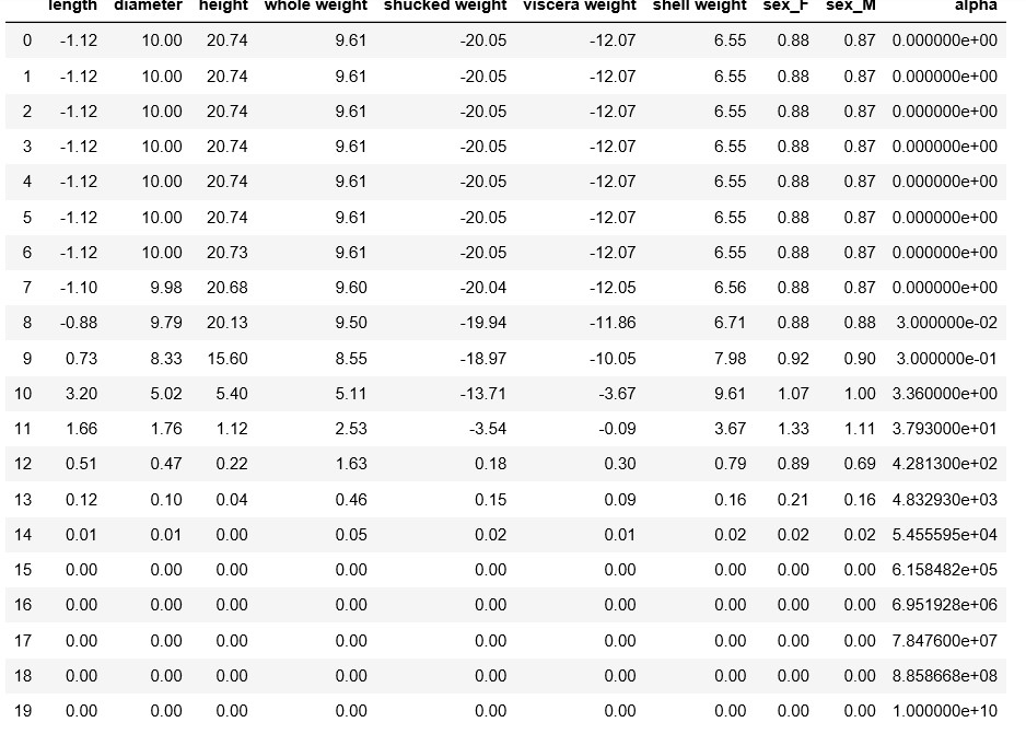
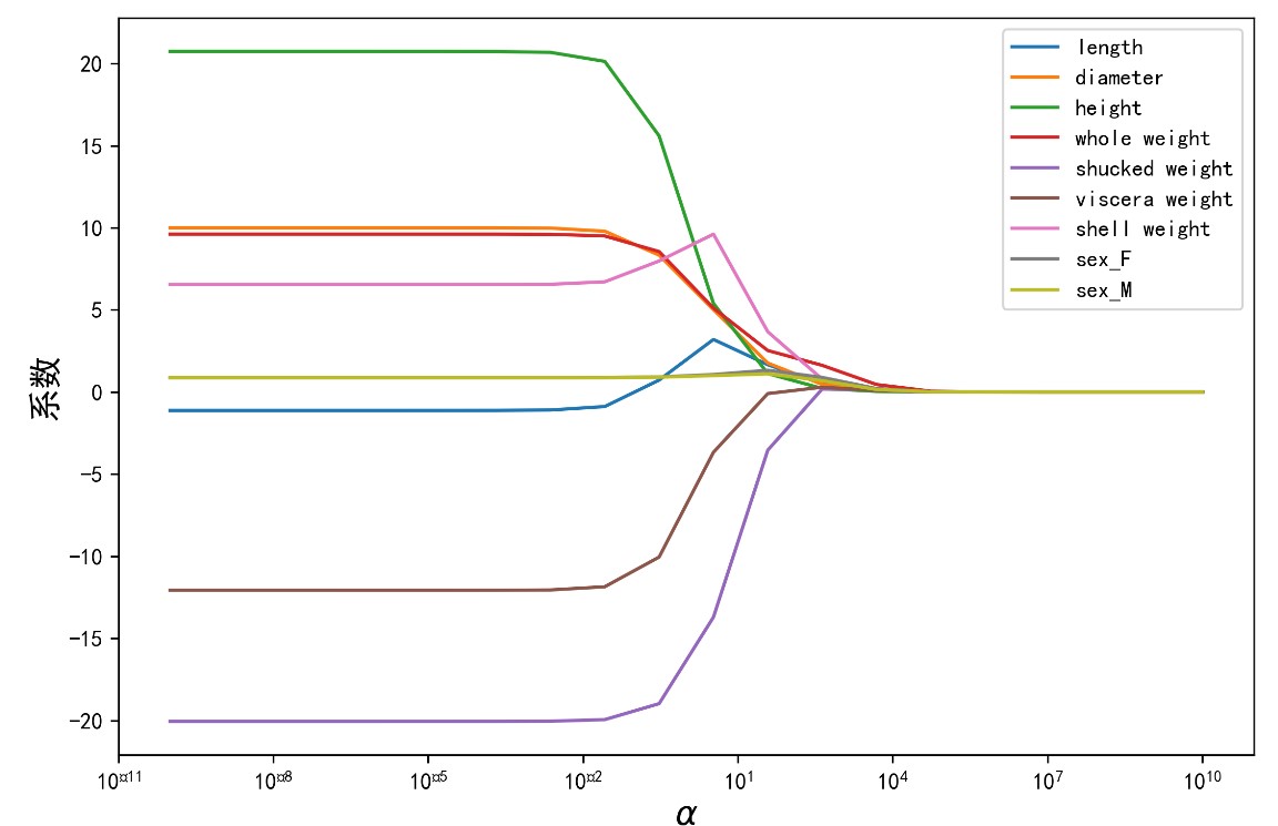
3.5 岭迹分析
alphas = np.logspace(-10,10,20)
coef = pd.DataFrame()
for alpha in alphas:
    ridge_clf = Ridge(alpha=alpha)
    ridge_clf.fit(X_train[features_without_ones],y_train)
    df = pd.DataFrame([ridge_clf.coef_],columns=X_train[features_without_ones].columns)
    df['alpha'] = alpha
    coef = coef.append(df,ignore_index=True)
coef.round(decimals=2)
import matplotlib.pyplot as plt
%matplotlib inline

plt.rcParams['font.sans-serif'] = ['SimHei','Times New Roman']
plt.rcParams['axes.unicode_minus'] = False

plt.rcParams['figure.dpi'] = 300
plt.figure(figsize=(9, 6))
coef['alpha'] = coef['alpha']

for feature in X_train.columns[:-1]:
    plt.plot('alpha',feature,data=coef)
ax = plt.gca()
ax.set_xscale('log')
plt.legend(loc='upper right')
plt.xlabel(r'$\alpha$',fontsize=15)
plt.ylabel('系数',fontsize=15)
plt.show()
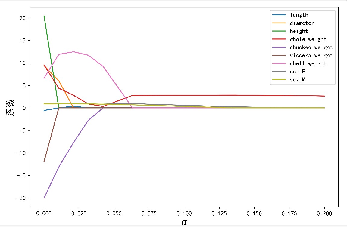
4 使用LASSO 构建鲍鱼年龄预测模型
from sklearn.linear_model import Lasso
lasso = Lasso(alpha=0.01)
lasso.fit(X_train[features_without_ones],y_train)
print(lasso.coef_)
print(lasso.intercept_)

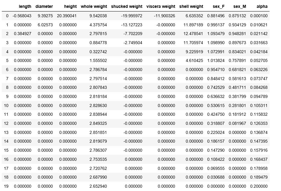
coef = pd.DataFrame()
for alpha in np.linspace(0.0001,0.2,20):
    lasso_clf = Lasso(alpha=alpha)
    lasso_clf.fit(X_train[features_without_ones],y_train)
    df = pd.DataFrame([lasso_clf.coef_],columns=X_train[features_without_ones].columns)
    df['alpha'] = alpha
    coef = coef.append(df,ignore_index=True)
coef.head()

plt.figure(figsize=(9, 6),dpi=600)
for feature in X_train.columns[:-1]:
    plt.plot('alpha',feature,data=coef)
plt.legend(loc='upper right')
plt.xlabel(r'$\alpha$',fontsize=15)
plt.ylabel('系数',fontsize=15)
plt.show()
coef
5 鲍鱼年龄预测模型效果评估
from sklearn.metrics import mean_squared_error
from sklearn.metrics import mean_absolute_error
from sklearn.metrics import r2_score
y_test_pred_lr = lr.predict(X_test.iloc[:,:-1])
print(round(mean_absolute_error(y_test,y_test_pred_lr),4))
y_test_pred_ridge = ridge.predict(X_test[features_without_ones])
print(round(mean_absolute_error(y_test,y_test_pred_ridge),4))
y_test_pred_lasso = lasso.predict(X_test[features_without_ones])
print(round(mean_absolute_error(y_test,y_test_pred_lasso),4))
1.6016
1.5984
1.6402
y_test_pred_lr = lr.predict(X_test.iloc[:,:-1])
print(round(mean_absolute_error(y_test,y_test_pred_lr),4))
y_test_pred_ridge = ridge.predict(X_test[features_without_ones])
print(round(mean_absolute_error(y_test,y_test_pred_ridge),4))
y_test_pred_lasso = lasso.predict(X_test[features_without_ones])
print(round(mean_absolute_error(y_test,y_test_pred_lasso),4))
5.3009
4.959
5.1
print(round(r2_score(y_test,y_test_pred_lr),4))
print(round(r2_score(y_test,y_test_pred_ridge),4))
print(round(r2_score(y_test,y_test_pred_lasso),4))
0.5257
0.5563
0.5437
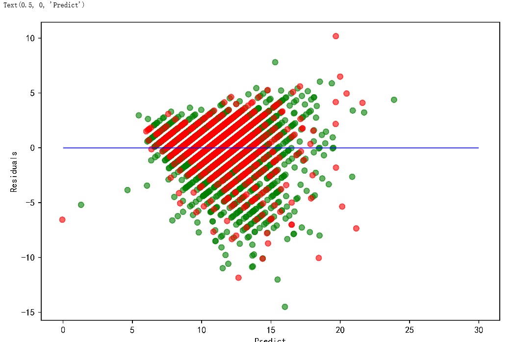
5.2 残差图
残差图是一种用来诊断回归模型效果的图。在残差图中,如果点随机分布在0附近,则说明回归效果较好。如果在残差图中发现了某种结构,则说明回归效果不佳,需要重新建模。
plt.figure(figsize=(9, 6),dpi=600)
y_train_pred_ridge = ridge.predict(X_train[features_without_ones])
plt.scatter(y_train_pred_ridge,y_train_pred_ridge - y_train,c="g",alpha=0.6)
plt.scatter(y_test_pred_ridge,y_test_pred_ridge - y_test,c="r",alpha=0.6)
plt.hlines(y=0,xmin=0,xmax=30,color="b",alpha=0.6)
plt.ylabel("Residuals")
plt.xlabel("Predict")
Original: https://blog.csdn.net/weixin_46728800/article/details/115571867
Author: Serendipity-垚
Title: 回归综合案例——利用回归模型预测鲍鱼年龄
原创文章受到原创版权保护。转载请注明出处:https://www.johngo689.com/696063/
转载文章受原作者版权保护。转载请注明原作者出处!