

转录因子分析可以了解细胞异质性背后的基因调控网络的异质性。转录因子分析也是单细胞转录组常见的分析内容,R语言分析一般采用的是SCENIC包,具体原理可参考两篇文章。1、《SCENIC : single-cell regulatory networkinference and clustering》。2、《Ascalable SCENIC workflow for single-cell gene regulatory network analysis》。 但是说在前头,SCENIC的计算量超级大,非常耗费内存和时间,如非必要,不要用一般的电脑分析尝试。可以借助服务器完成分析,或者减少分析细胞数,再或者使用SCENIC的Python版本。这里我们也是仅仅进行演示,数据没有实际意义,人为减少了基因与细胞,然而就这也很费时间。重要的是看看流程。
首先开始前,需要做两件事。第一毫无疑问是安装和加载R包,需要的比较多,如果没有请安装。第二则是下载基因注释配套数据库。
library(Seurat)
library(tidyverse)
library(foreach)
library(RcisTarget)
library(doParallel)
library(SCopeLoomR)
library(AUCell)
BiocManager::install(c("doMC", "doRNG"))
library(doRNG)
BiocManager::install("GENIE3")
library(GENIE3)
#if (!requireNamespace("devtools", quietly = TRUE))
devtools::install_github("aertslab/SCENIC")
packageVersion("SCENIC")
library(SCENIC)
#这里下载人的
dbFiles <- c("https: resources.aertslab.org cistarget databases homo_sapiens hg19 refseq_r45 mc9nr gene_based hg19-500bp-upstream-7species.mc9nr.feather", "https: hg19-tss-centered-10kb-7species.mc9nr.feather") for(featherurl in dbfiles) { download.file(featherurl, destfile="basename(featherURL))" } < code></->
接着就是构建分析文件。
#构建分析数据
exprMat <- as.matrix(immune@assays$rna@data)#表达矩阵 exprmat[1:4,1:4]#查看数据 cellinfo <- immune@meta.data[,c("celltype","ncount_rna","nfeature_rna")] colnames(cellinfo) c('celltype', 'ngene' ,'numi') head(cellinfo) table(cellinfo$celltype) #构建scenicoptions对象,接下来的scenic分析都是基于这个对象的信息生成的 scenicoptions initializescenic(org="hgnc" , dbdir="F:/cisTarget_databases" ncores="1)" < code></->
构建共表达网络,最后一步很费时间。
Co-expression network
genesKept <- 1 2 3 4 5 6 7 8 9 10 676 1839 genefiltering(exprmat, scenicoptions) exprmat.filtered <- exprmat[geneskept, ] exprmat.filtered[1:4,1:4] runcorrelation(exprmat.filtered, exprmat.filtered.log log2(exprmat.filtered + 1) rungenie3(exprmat.filtered.log, #using tfs as potential regulators... #running genie3 part #finished running genie3. #warning message: #in : # only (37%) of the in database were found dataset. do they use same gene ids? < code></->
构建基因调控网络GRN并进行AUC评分。也是耗费时间的过程。运行完成的结果就是整个分析得到的内容,需要按照自己的目的去筛选。
Build and score the GRN
scenicOptions <- runscenic_1_coexnetwork2modules(scenicoptions) scenicoptions <- runscenic_2_createregulons(scenicoptions) exprmat_log log2(exprmat + 1) runscenic_3_scorecells(scenicoptions,exprmat_log) runscenic_4_aucell_binarize(scenicoptions) saverds(scenicoptions, file="int/scenicOptions.Rds" ) < code></->
以下是运行记录
>scenicOptions <- 1 2 3 13 27 149 174 236 436 500 523 617 671 676 12551 22290 1993247 runscenic_2_createregulons(scenicoptions) 13:21 step 2. identifying regulons tfmodulessummary: [,1] top5pertargetandtop3sd top5pertargetandtop50 top1sdandtop10pertarget top50pertargetandtop1sd top50andtop10pertarget w0.005 w0.005andtop1sd top50pertarget top50andtop3sd top3sd top50 w0.005andtop50pertarget top1sd top5pertarget top10pertarget w0.001 rcistarget: calculating auc scoring database: [source file: hg19-500bp-upstream-7species.mc9nr.feather] hg19-tss-centered-10kb-7species.mc9nr.feather] not all characters in c: users liuhl desktop 1.r could be decoded using cp936. to try a different encoding, choose "file | reopen with encoding..." from the main menu.17:17 adding motif annotation biocparallel... number of motifs initial enrichment: annotated matching tf: 17:38 pruning targets 19:04 that support regulons: preview enrichment saved as: output step2_motifenrichment_preview.html there were warnings (use warnings() see them)> exprMat_log <- log2(exprmat + 1)> scenicOptions <- 318 runscenic_3_scorecells(scenicoptions,exprmat_log) 19:06 step 3. analyzing the network activity in each individual cell number of regulons to evaluate on cells: biggest (non-extended) regulons: elf1 (1760g) ets1 (1734g) fli1 (1604g) elk3 (1493g) polr2a (1453g) chd2 (1251g) etv3 (1249g) elk4 (1148g) taf1 (974g) erg (956g) quantiles for genes detected by cell: (non-detected are shuffled at end ranking. keep it mind when choosing threshold calculating auc). min 1% 5% 10% 50% 100% 205.00 224.76 276.90 321.40 695.00 997.00 warning .aucell_calcauc(genesets="geneSets," rankings="rankings," ncores="nCores," : using only first (aucmaxrank) calculate auc. 19:07 finished running aucell. plotting heatmap... t-snes... message: max(denscurve$y[nextmaxs]) max里所有的参数都不存在;回覆-inf> scenicOptions <- 168 207 439 runscenic_4_aucell_binarize(scenicoptions) binary regulon activity: tf regulons x cells. (299 including 'extended' versions) are active in more than 1% (4.39)> saveRDS(scenicOptions, file = "int/scenicOptions.Rds")
</-></-></-></->
每一步的分析结果SCENIC都会自动保存在所创建的int和out文件夹。接下来对结果进行可视化,这里是随机选的,没有生物学意义。实际情况是要根据自己的研究目的。
1、可视化转录因子与seurat细胞分群联动
#regulons AUC
AUCmatrix <- readrds("int 3.4_regulonauc.rds") aucmatrix <- aucmatrix@assays@data@listdata$auc data.frame(t(aucmatrix), check.names="F)" regulonname_auc colnames(aucmatrix) gsub(' \\(','_',regulonname_auc) gsub('\\)','',regulonname_auc) scrnaauc addmetadata(immune, aucmatrix) scrnaauc@assays$integrated null saverds(scrnaauc,'immuneauc.rds') #二进制regulo auc binmatrix 4.1_binaryregulonactivity.rds") data.frame(t(binmatrix), regulonname_bin colnames(binmatrix) \\(','_',regulonname_bin) gsub('\\)','',regulonname_bin) scrnabin binmatrix) scrnabin@assays$integrated saverds(scrnabin, 'immunebin.rds') < code></->
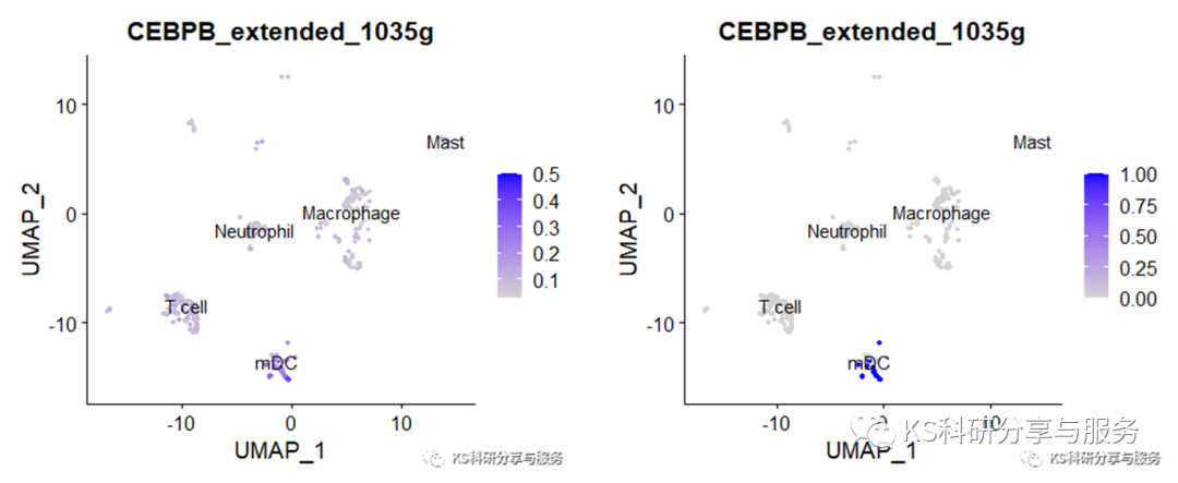
作图使用Seurat中FeaturePlot函数。小提琴图也是可以的。
FeaturePlot(scRNAauc, features='CEBPB_extended_1035g', label=T, reduction = 'umap')
FeaturePlot(scRNAbin, features='CEBPB_extended_1035g', label=T, reduction = 'umap')

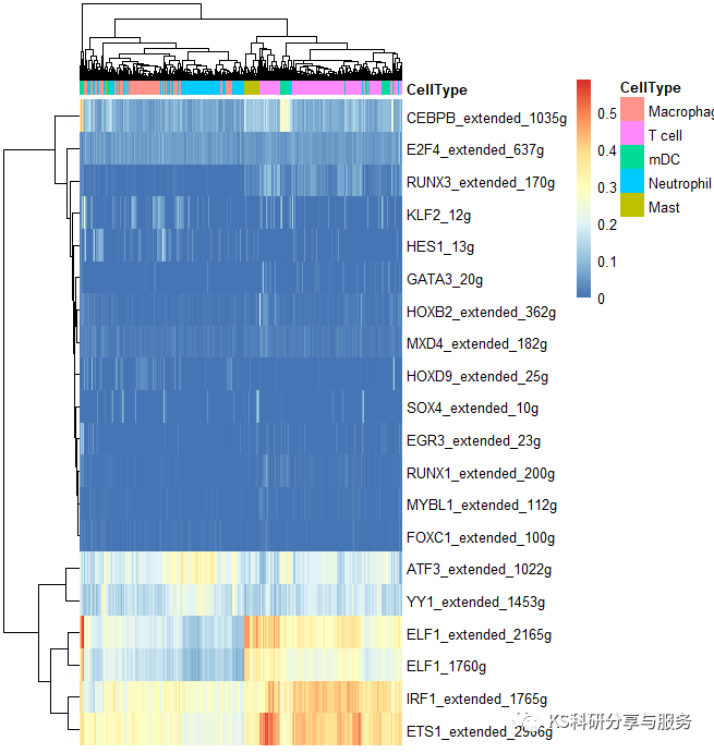
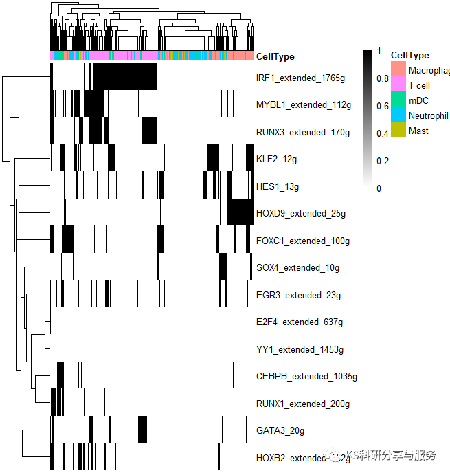
2、最常见的热图,选择需要可视化的regulons。
library(pheatmap)
celltype = subset(cellInfo,select = 'CellType')
AUCmatrix <- t(aucmatrix) binmatrix <- t(binmatrix) regulons c('cebpb_extended_1035g','runx1_extended_200g', 'foxc1_extended_100g','mybl1_extended_112g', 'irf1_extended_1785g', 'elf1_1760g','elf1_extended_2165g', 'irf1_extended_1765g','ets1_extended_2906g', 'yy1_extended_1453g','atf3_extended_1022g', 'e2f4_extended_637g', 'klf2_12g','hes1_13g', 'gata3_20g','hoxb2_extended_362g', 'sox4_extended_10g', 'runx3_extended_170g','egr3_extended_23g', 'mxd4_extended_182g','hoxd9_extended_25g') aucmatrix aucmatrix[rownames(aucmatrix)%in%regulons,] binmatrix[rownames(binmatrix)%in%regulons,] pheatmap(aucmatrix, show_colnames="F," annotation_col="celltype," width="6," height="5)" pheatmap(binmatrix, color="colorRampPalette(colors" = c("white","black"))(100), < code></->
好了,以上是一个基本的流程演示,具体怎么用这个结果,如何解读,可以参考相关的高分文献,了解分析原理,与自己的研究相结合。
更多精彩内容请访问我的个人公众号《KS科研分享与服务》!
Original: https://blog.csdn.net/qq_42090739/article/details/123701891
Author: TS的美梦
Title: 跟着Cell学单细胞转录组分析(十二):转录因子分析
原创文章受到原创版权保护。转载请注明出处:https://www.johngo689.com/694997/
转载文章受原作者版权保护。转载请注明原作者出处!