神经网络1.1 感知机模型(神经元模型)

1.激活函数

1.1 Sigmoid函数

Sigmoid 是常用的非线性的激活函数，表达式如下：
f ( x ) = 1 1 + e − x f(x) = \frac{1}{1 + e^{-x}}f (x )=1 +e −x 1 ​

• 特性：它能够把输入的连续实值变换为0 0 0和1 1 1之间的输出，特别的，如果是非常大的负数，那么输出就是0 0 0；如果是非常大的正数，输出就是1 1 1.

• 缺点：在深度神经网络中梯度反向传递时导致梯度爆炸和梯度消失，其中梯度爆炸发生的概率非常小，而梯度消失发生的概率比较大。

1.2 tanh函数

tanh函数也是非线性函数，其函数解析式为：
t a n h ( x ) = e x − e − x e x + e − x tanh(x) = \frac{e^x – e^{-x}}{e^x + e^{-x}}t a n h (x )=e x +e −x e x −e −x ​
tanh读作 Hyperbolic Tangent，它解决了 Sigmoid函数的不是 zero-centered输出问题，然而，梯度消失(gradient vanishing)的问题和幂运算的问题仍然存在。

1.3 Relu函数

Relu函数实际上就是个取最大值函数，其函数解析式如下所示：
f ( x ) = max ⁡ ( 0 , x ) f(x) = \max{(0, x)}f (x )=max (0 ,x )

• Relu是目前最常用的激活函数，一般搭建人工神经网络时推荐优先尝试
• Relu并非全区间可导，但我们可以取 sub-gradient
  *
• 解决了 gradient vanishing问题 (在正区间)
• 计算速度非常快，只需要判断输入是否大于0 0 0
• 收敛速度远快于 Sigmoid和 tanh
  *
• ReLU的输出不是 zero-centered
• Dead ReLU Problem，指的是某些神经元可能永远不会被激活，导致相应的参数永远不能被更新。有两个主要原因可能导致这种情况产生: (1) 非常不幸的参数初始化，这种情况比较少见 (2) learning rate太高导致在训练过程中参数更新太大，不幸使网络进入这种状态。解决方法是可以采用Xavier初始化方法，以及避免将 learning rate设置太大或使用 adagrad等自动调节 learning rate的算法。

1.4 Leaky ReLU函数(PReLU)

函数表达式：
f ( x ) = max ⁡ ( α x , x ) f(x) = \max(\alpha x, x)f (x )=max (αx ,x )
人们为了解决 Dead ReLU Problem，提出了将ReLU的前半段设为α x \alpha x αx而非0 0 0，通常α = 0.01 \alpha=0.01 α=0 .0 1。另外一种直观的想法是基于参数的方法，即P a r a m e t r i c R e L U : f ( x ) = max ⁡ ( α x , x ) Parametric ReLU:f(x) = \max(\alpha x, x)P a r a m e t r i c R e L U :f (x )=max (αx ,x )，其中α \alpha α
可由方向传播算法学出来。理论上来讲， Leaky ReLU有 ReLU的所有优点，外加不会有 Dead ReLU问题，但是在实际操作当中，并没有完全证明 Leaky ReLU总是好于 ReLU。

1.5 ELU(Exponential Linear Units) 函数

函数表达式：
f ( x ) = { x , i f x > 0 α ( e x − 1 ) , o t h e r w i s e f(x) = \left{\begin{matrix} x ,&if\ x > 0\ \alpha(e^x – 1), &otherwise \end{matrix}\right.f (x )={x ,α(e x −1 ),​i f x >0 o t h e r w i s e ​
ELU不会有 Dead ReLU问题 输出的均值接近0 0 0， zero-centered。但计算量偏大，在目前的实际应用中并未被证明总是好于 ReLU。

1.6 UnitStep 阶跃函数

函数表达式：
f ( x ) = { 1 , i f x > 0 0 , o t h e r w i s e f(x) = \left{\begin{matrix} 1 ,&if\ x > 0\ 0, &otherwise \end{matrix}\right.f (x )={1 ,0 ,​i f x >0 o t h e r w i s e ​
传统的阶跃函数，不连续，因此难以进行数学分析。常用其它连续可导函数代替。

2.感知机模型(神经元模型)

设输入空间(特征空间)为X ⊆ R n X\subseteq\R^n X ⊆R n，输出空间为Y = { 0 , 1 } Y = {0, 1}Y ={0 ,1 }

输入x ∈ X x \in X x ∈X为实例的特征向量，输出y ∈ Y y \in Y y ∈Y为实例的类别

由输入空间到输出空间的如下函数称为感知机：
f ( x ) = s i g n ( w x + b ) f(x) = sign(wx + b)f (x )=s i g n (w x +b )
其中w w w和b b b为模型参数，w ∈ R n w \in \R^n w ∈R n称为权值，b ∈ R b \in \R b ∈R称为偏置。s i g n sign s i g n是符号函数。

假设我们目前的任务是通过感知机对具有n n n维特征的向量进行分类。我们可以将该感知机的模型视作一个神经元模型。n n n维向量(( x 1 , x 2 , … , x n ) (x_1, x_2, \dots, x_n)(x 1 ​,x 2 ​,…,x n ​))对应的是神经元的n n n个输入。

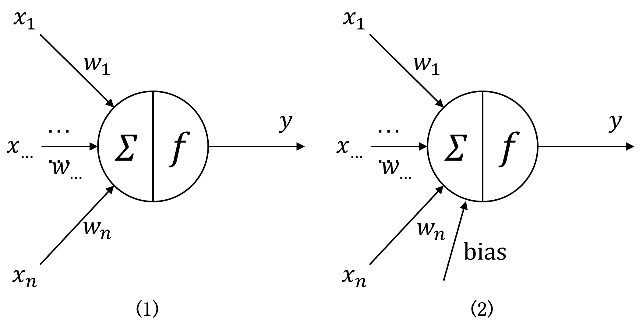
我们对这n n n个输入分别乘其对应的权值后求和，经过激活函数后得到分类结果。

但是我们注意到，当神经网络的输入向量为0 0 0时，会产生激活失败误分类的情况，为了避免这种情况，我们对其加偏置项后再进入激活函数，也就是感知机模型中的b b b。

我们首先对输入向量乘对应的权值加偏置项后得到∑ k = 1 k ≤ n w x i + b \sum_{k = 1}^{k \leq n} wx_i + b ∑k =1 k ≤n ​w x i ​+b，将其经过激活函数后与标签进行比对，并根据是否与标签相等来更新参数的值：
w = w + α × ( y − y ^ ) × x b = b + α × ( y − y ^ ) w = w + \alpha \times(y – \hat{y})\times x \ b = b + \alpha \times (y – \hat{y})w =w +α×(y −y ^​)×x b =b +α×(y −y ^​)
其中α \alpha α为步长，又称学习率。以上过程对所有训练数据执行一次后，可以得到一轮训练后的w w w和b b b。

显然，由于权值参数对应于n n n维特征向量，因此w w w的维度一定与输入向量的特征维数有关。

此处给出基于 Python实现的感知机模型。

import numpy as np
import matplotlib.pyplot as plt

class ActivateFunction(object):
    @staticmethod
    def Sigmoid(x):
        return (1 / (1 + np.exp(-x)))
    @staticmethod
    def ReLu(x):
        if x  0: return 0
        else: return x

    @staticmethod
    def Softmax(x):
        return np.exp(x) / np.sum(np.exp(x))
    @staticmethod
    def UnitStep(x):
        return 1 if x > 0 else 0

class Perceptron(object):

    def __init__(self, input_num, activator):
        self.activator = activator
        self.size = input_num
        self.weights = [0.0 for i in range(input_num)]
        self.bias = 0.0

    def Predict(self, input_vec):
        return self.activator(np.dot(input_vec, self.weights) + self.bias)

    def SingleIteration(self, input_vecs, labels, rate):
        samples = zip(input_vecs, labels)
        for (input_vec, label) in samples:
            output = self.Predict(input_vec)
            delta = label - output
            input_vec = np.array(input_vec)
            self.weights += rate * delta * input_vec
            self.bias += rate * delta

    def fit(self, input_vecs, labels, iteration, rate):
        input_vecs, labels = np.array(input_vecs), np.array(labels)
        for i in range(iteration):
            self.SingleIteration(input_vecs, labels, rate)

    def GetParameters(self):
        return self.weights, self.bias

if __name__ == "__main__":
    data, label = [], []
    file = open(r'.\Python\x.txt')
    for line in file.readlines():
        line_data = line.strip().split(',')
        data.append([float(line_data[0]), float(line_data[1])])
    file.close()
    file = open(r'.\Python\y.txt')
    for line in file.readlines():
        line_data = line.strip().split(',')
        label = list(map(int, line_data))
    file.close

    p = Perceptron(2, ActivateFunction.UnitStep)
    p.fit(data, label, 1000, 0.1)
    w, b = p.GetParameters()
    x1 = np.arange(-5, 10, 0.1)
    x2 = (w[0] * x1 + b) / (-w[1])

    data = np.array(data)
    label = np.array(label)
    idx_p = np.where(label == 1)
    idx_n = np.where(label != 1)
    data_p = data[idx_p]
    data_n = data[idx_n]

    plt.scatter(data_p[:, 0], data_p[:, 1], color='red')
    plt.scatter(data_n[:, 0], data_n[:, 1], color='blue')
    plt.plot(x1, x2)
    plt.show()

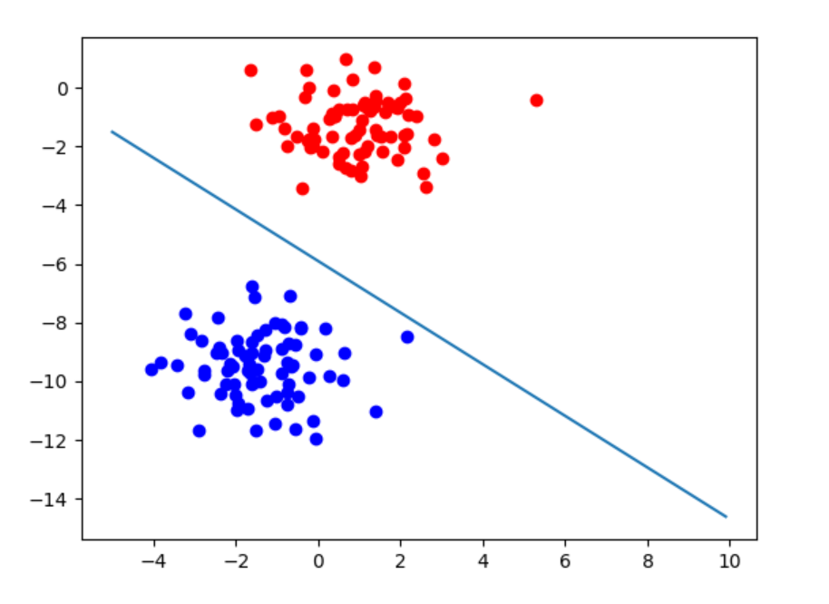
分类效果示例如上所示。

Original: https://blog.csdn.net/yanweiqi1754989931/article/details/123465547
Author: HeartFireY
Title: 神经网络1.1 感知机模型(神经元模型)