

往期学习资料推荐:
本系列目录:
后续继续更新!!!!
1 深度学习步骤
(1)数据预处理:通过专门的数据加载,通过批训练提高模型表现,每次训练读取固定数量的样本输入到模型中进行训练
(2)深度神经网络搭建:逐层搭建,实现特定功能的层(如积层、池化层、批正则化层、LSTM层等)
(3)损失函数和优化器的设定:保证反向传播能够在用户定义的模型结构上实现
(4)模型训练:使用并行计算加速训练,将数据按批加载,放入GPU中训练,对损失函数反向传播回网络最前面的层,同时使用优化器调整网络参数
2 基本配置
-
导入相关的包
-
统一设置超参数:batch size、初始学习率、训练次数、GPU配置
3 数据读入
- 读取方式:通过Dataset+DataLoader的方式加载数据,Dataset定义好数据的格式和数据变换形式,DataLoader用iterative的方式不断读入批次数据。
- 自定义Dataset类:实现
__init___、__getitem__、__len__函数 torch.utils.data.DataLoader参数:- batch_size:样本是按”批”读入的,表示每次读入的样本数
- num_workers:表示用于读取数据的进程数
- shuffle:是否将读入的数据打乱
- drop_last:对于样本最后一部分没有达到批次数的样本,使其不再参与训练
4 模型构建
通过 Module类构造模型,实例化模型之后,可完成模型构造
- 不含模型参数的层
tensor([-10., -5., 0., 5., 10.])
- 含模型参数的层:如果一个
Tensor是Parameter,那么它会⾃动被添加到模型的参数列表里
MyListDense(
  (params): ParameterList(
      (0): Parameter containing: [torch.FloatTensor of size 4x4]
      (1): Parameter containing: [torch.FloatTensor of size 4x4]
      (2): Parameter containing: [torch.FloatTensor of size 4x4]
      (3): Parameter containing: [torch.FloatTensor of size 4x1]
  )
)
MyDictDense(
  (params): ParameterDict(
      (linear1): Parameter containing: [torch.FloatTensor of size 4x4]
      (linear2): Parameter containing: [torch.FloatTensor of size 4x1]
      (linear3): Parameter containing: [torch.FloatTensor of size 4x2]
  )
)
- 二维卷积层:使用
nn.Conv2d类构造,模型参数包括卷积核和标量偏差,在训练模式时,通常先对卷积核随机初始化,再不断迭代卷积核和偏差
torch.Size([8, 8])
- 池化层:直接计算池化窗口内元素的最大值或者平均值,分别叫做最大池化或平均池化
tensor([[4., 5.],
        [7., 8.]])
pool2d(X, (2, 2), 'avg')
tensor([[2., 3.],
        [5., 6.]])
- 神经网络训练过程:
- 定义可学习参数的神经网络
- 在输入数据集上进行迭代训练
- 通过神经网络处理输入数据
- 计算loss(损失值)
- 将梯度反向传播给神经网络参数
- 更新网络参数,使用梯度下降
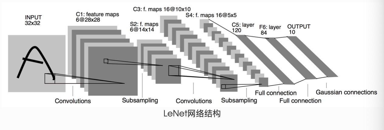
- LeNet(前馈神经网络)

import torch.nn.functional as F

class Net(nn.Module):
    def __init__(self):
        super(Net, self).__init__()
        # 输入图像channel是1;输出channel是6;5x5卷积核
        self.conv1 = nn.Conv2d(1, 6, 5)
        self.conv2 = nn.Conv2d(6, 16, 5)
        # an affine operation: y = Wx + b
        self.fc1 = nn.Linear(16 * 5 * 5, 120)
        self.fc2 = nn.Linear(120, 84)
        self.fc3 = nn.Linear(84, 10)

    def forward(self, x):
        # 2x2 Max pooling
        x = F.max_pool2d(F.relu(self.conv1(x)), (2, 2))
        # 如果是方阵,则可以只使用一个数字进行定义
        x = F.max_pool2d(F.relu(self.conv2(x)), 2)
        x = x.view(-1, self.num_flat_features(x))
        x = F.relu(self.fc1(x))
        x = F.relu(self.fc2(x))
        x = self.fc3(x)
        return x

    def num_flat_features(self, x):
        # 除去批处理维度的其他所有维度
        size = x.size()[1:]
        num_features = 1
        for s in size:
            num_features *= s
        return num_features

net = Net()
net
Net(
  (conv1): Conv2d(1, 6, kernel_size=(5, 5), stride=(1, 1))
  (conv2): Conv2d(6, 16, kernel_size=(5, 5), stride=(1, 1))
  (fc1): Linear(in_features=400, out_features=120, bias=True)
  (fc2): Linear(in_features=120, out_features=84, bias=True)
  (fc3): Linear(in_features=84, out_features=10, bias=True)
)
tensor([[-0.0921, -0.0605, -0.0726, -0.0451,  0.1399, -0.0087,  0.1075,  0.0799,
         -0.1472,  0.0288]], grad_fn=<addmmbackward>)</addmmbackward>
清零所有参数的梯度缓存,然后进行随机梯度的反向传播
net.zero_grad()
out.backward(torch.randn(1, 10))
- AlexNet
class AlexNet(nn.Module):
    def __init__(self):
        super(AlexNet, self).__init__()
        self.conv = nn.Sequential(
            # in_channels, out_channels, kernel_size, stride, padding
            nn.Conv2d(1, 96, 11, 4),
            nn.ReLU(),
            # kernel_size, stride
            nn.MaxPool2d(3, 2),
            # 减小卷积窗口,使用填充为2来使得输入与输出的高和宽一致,且增大输出通道数
            nn.Conv2d(96, 256, 5, 1, 2),
            nn.ReLU(),
            nn.MaxPool2d(3, 2),
            # 连续3个卷积层,且使用更小的卷积窗口。
            # 除了最后的卷积层外,进一步增大了输出通道数。
            # 前两个卷积层后不使用池化层来减小输入的高和宽
            nn.Conv2d(256, 384, 3, 1, 1),
            nn.ReLU(),
            nn.Conv2d(384, 384, 3, 1, 1),
            nn.ReLU(),
            nn.Conv2d(384, 256, 3, 1, 1),
            nn.ReLU(),
            nn.MaxPool2d(3, 2)
        )
         # 这里全连接层的输出个数比LeNet中的大数倍。使用丢弃层来缓解过拟合
        self.fc = nn.Sequential(
            nn.Linear(256*5*5, 4096),
            nn.ReLU(),
            nn.Dropout(0.5),
            nn.Linear(4096, 4096),
            nn.ReLU(),
            nn.Dropout(0.5),
            # 输出层。由于这里使用Fashion-MNIST,所以用类别数为10,而非论文中的1000
            nn.Linear(4096, 10),
        )

    def forward(self, img):
        feature = self.conv(img)
        output = self.fc(feature.view(img.shape[0], -1))
        return output
net = AlexNet()
print(net)
AlexNet(
  (conv): Sequential(
    (0): Conv2d(1, 96, kernel_size=(11, 11), stride=(4, 4))
    (1): ReLU()
    (2): MaxPool2d(kernel_size=3, stride=2, padding=0, dilation=1, ceil_mode=False)
    (3): Conv2d(96, 256, kernel_size=(5, 5), stride=(1, 1), padding=(2, 2))
    (4): ReLU()
    (5): MaxPool2d(kernel_size=3, stride=2, padding=0, dilation=1, ceil_mode=False)
    (6): Conv2d(256, 384, kernel_size=(3, 3), stride=(1, 1), padding=(1, 1))
    (7): ReLU()
    (8): Conv2d(384, 384, kernel_size=(3, 3), stride=(1, 1), padding=(1, 1))
    (9): ReLU()
    (10): Conv2d(384, 256, kernel_size=(3, 3), stride=(1, 1), padding=(1, 1))
    (11): ReLU()
    (12): MaxPool2d(kernel_size=3, stride=2, padding=0, dilation=1, ceil_mode=False)
  )
  (fc): Sequential(
    (0): Linear(in_features=6400, out_features=4096, bias=True)
    (1): ReLU()
    (2): Dropout(p=0.5, inplace=False)
    (3): Linear(in_features=4096, out_features=4096, bias=True)
    (4): ReLU()
    (5): Dropout(p=0.5, inplace=False)
    (6): Linear(in_features=4096, out_features=10, bias=True)
  )
)
5 损失函数
- 二分类交叉熵损失函数:
torch.nn.BCELoss,用于计算二分类任务时的交叉熵
m = nn.Sigmoid()
loss = nn.BCELoss()
input = torch.randn(3, requires_grad=True)
target = torch.empty(3).random_(2)

output = loss(m(input), target)
output.backward()
print('BCE损失函数的计算结果:',output)
BCE损失函数的计算结果: tensor(0.9389, grad_fn=<binarycrossentropybackward>)</binarycrossentropybackward>
- 交叉熵损失函数:
torch.nn.CrossEntropyLoss,用于计算交叉熵
loss = nn.CrossEntropyLoss()
input = torch.randn(3, 5, requires_grad=True)
target = torch.empty(3, dtype=torch.long).random_(5)

output = loss(input, target)
output.backward()
print('CrossEntropy损失函数的计算结果:',output)
CrossEntropy损失函数的计算结果: tensor(2.7367, grad_fn=<nlllossbackward>)</nlllossbackward>
- L1损失函数:
torch.nn.L1Loss,用于计算输出y和真实值target之差的绝对值
loss = nn.L1Loss()
input = torch.randn(3, 5, requires_grad=True)
target = torch.randn(3, 5)

output = loss(input, target)
output.backward()
print('L1损失函数的计算结果:',output)
L1损失函数的计算结果: tensor(1.0351, grad_fn=<l1lossbackward>)</l1lossbackward>
- MSE损失函数:
torch.nn.MSELoss,用于计算输出y和真实值target之差的平方
loss = nn.MSELoss()
input = torch.randn(3, 5, requires_grad=True)
target = torch.randn(3, 5)

output = loss(input, target)
output.backward()
print('MSE损失函数的计算结果:',output)
MSE损失函数的计算结果: tensor(1.7612, grad_fn=<mselossbackward>)</mselossbackward>
- 平滑L1(Smooth L1)损失函数:
torch.nn.SmoothL1Loss,用于计算L1的平滑输出,减轻离群点带来的影响,通过与L1损失的比较,在0点的尖端处,过渡更为平滑
loss = nn.SmoothL1Loss()
input = torch.randn(3, 5, requires_grad=True)
target = torch.randn(3, 5)

output = loss(input, target)
output.backward()
print('Smooth L1损失函数的计算结果:',output)
Smooth L1损失函数的计算结果: tensor(0.7252, grad_fn=<smoothl1lossbackward>)</smoothl1lossbackward>
- 目标泊松分布的负对数似然损失:
torch.nn.PoissonNLLLoss
loss = nn.PoissonNLLLoss()
log_input = torch.randn(5, 2, requires_grad=True)
target = torch.randn(5, 2)

output = loss(log_input, target)
output.backward()
print('PoissonNL损失函数的计算结果:',output)
PoissonNL损失函数的计算结果: tensor(1.7593, grad_fn=<meanbackward0>)</meanbackward0>
- KL散度:
torch.nn.KLDivLoss,用于连续分布的距离度量,可用在对离散采用的连续输出空间分布的回归场景
inputs = torch.tensor([[0.5, 0.3, 0.2], [0.2, 0.3, 0.5]])
target = torch.tensor([[0.9, 0.05, 0.05], [0.1, 0.7, 0.2]], dtype=torch.float)
loss = nn.KLDivLoss(reduction='batchmean')

output = loss(inputs,target)
print('KLDiv损失函数的计算结果:',output)
KLDiv损失函数的计算结果: tensor(-1.0006)
- MarginRankingLoss:
torch.nn.MarginRankingLoss,用于计算两组数据之间的差异(相似度),可使用在排序任务的场景
loss = nn.MarginRankingLoss()
input1 = torch.randn(3, requires_grad=True)
input2 = torch.randn(3, requires_grad=True)
target = torch.randn(3).sign()

output = loss(input1, input2, target)
output.backward()
print('MarginRanking损失函数的计算结果:',output)
MarginRanking损失函数的计算结果: tensor(1.1762, grad_fn=<meanbackward0>)</meanbackward0>
- 多标签边界损失函数:
torch.nn.MultiLabelMarginLoss,用于计算多标签分类问题的损失
loss = nn.MultiLabelMarginLoss()
x = torch.FloatTensor([[0.9, 0.2, 0.4, 0.8]])
真实的分类是,第3类和第0类
y = torch.LongTensor([[3, 0, -1, 1]])

output = loss(x, y)
print('MultiLabelMargin损失函数的计算结果:',output)
MultiLabelMargin损失函数的计算结果: tensor(0.4500)
- 二分类损失函数:
torch.nn.SoftMarginLoss,用于计算二分类的logistic损失
定义两个样本,两个神经元
inputs = torch.tensor([[0.3, 0.7], [0.5, 0.5]])
target = torch.tensor([[-1, 1], [1, -1]], dtype=torch.float)

该loss对每个神经元计算,需要为每个神经元单独设置标签
loss_f = nn.SoftMarginLoss()
output = loss_f(inputs, target)
print('SoftMargin损失函数的计算结果:',output)
SoftMargin损失函数的计算结果: tensor(0.6764)
- 多分类的折页损失函数:
torch.nn.MultiMarginLoss,用于计算多分类问题的折页损失
inputs = torch.tensor([[0.3, 0.7], [0.5, 0.5]])
target = torch.tensor([0, 1], dtype=torch.long)

loss_f = nn.MultiMarginLoss()
output = loss_f(inputs, target)
print('MultiMargin损失函数的计算结果:',output)
MultiMargin损失函数的计算结果: tensor(0.6000)
- 三元组损失函数:
torch.nn.TripletMarginLoss,用于处理
triplet_loss = nn.TripletMarginLoss(margin=1.0, p=2)
anchor = torch.randn(100, 128, requires_grad=True)
positive = torch.randn(100, 128, requires_grad=True)
negative = torch.randn(100, 128, requires_grad=True)

output = triplet_loss(anchor, positive, negative)
output.backward()
print('TripletMargin损失函数的计算结果:',output)
TripletMargin损失函数的计算结果: tensor(1.1507, grad_fn=<meanbackward0>)</meanbackward0>
- HingEmbeddingLoss:
torch.nn.HingeEmbeddingLoss,用于计算输出的embedding结果的Hing损失
loss_f = nn.HingeEmbeddingLoss()
inputs = torch.tensor([[1., 0.8, 0.5]])
target = torch.tensor([[1, 1, -1]])

output = loss_f(inputs,target)
print('HingEmbedding损失函数的计算结果:',output)
HingEmbedding损失函数的计算结果: tensor(0.7667)
- 余弦相似度:
torch.nn.CosineEmbeddingLoss,用于计算两个向量的余弦相似度,如果两个向量距离近,则损失函数值小,反之亦然
loss_f = nn.CosineEmbeddingLoss()
inputs_1 = torch.tensor([[0.3, 0.5, 0.7], [0.3, 0.5, 0.7]])
inputs_2 = torch.tensor([[0.1, 0.3, 0.5], [0.1, 0.3, 0.5]])
target = torch.tensor([1, -1], dtype=torch.float)

output = loss_f(inputs_1,inputs_2,target)
print('CosineEmbedding损失函数的计算结果:',output)
CosineEmbedding损失函数的计算结果: tensor(0.5000)
- CTC损失函数:
torch.nn.CTCLoss,用于处理时序数据的分类问题,计算连续时间序列和目标序列之间的损失
Target are to be padded
序列长度
T = 50
类别数(包括空类)
C = 20
batch size
N = 16
Target sequence length of longest target in batch (padding length)
S = 30
Minimum target length, for demonstration purposes
S_min = 10

input = torch.randn(T, N, C).log_softmax(2).detach().requires_grad_()
初始化target(0 = blank, 1:C = classes)
target = torch.randint(low=1, high=C, size=(N, S), dtype=torch.long)

input_lengths = torch.full(size=(N,), fill_value=T, dtype=torch.long)
target_lengths = torch.randint(low=S_min, high=S, size=(N,), dtype=torch.long)

ctc_loss = nn.CTCLoss()
loss = ctc_loss(input, target, input_lengths, target_lengths)
loss.backward()
print('CTC损失函数的计算结果:',loss)
CTC损失函数的计算结果: tensor(6.1333, grad_fn=<meanbackward0>)</meanbackward0>
6 优化器
- 使用方向:为了使求解参数过程更快,使用BP+优化器逼近求解
- Optimizer的属性:
defaults:优化器的超参数state:参数的缓存param_groups:参数组,顺序是params,lr,momentum,dampening,weight_decay,nesterov- Optimizer的方法:
zero_grad():清空所管理参数的梯度step():执行一步梯度更新add_param_group():添加参数组load_state_dict():加载状态参数字典,可以用来进行模型的断点续训练,继续上次的参数进行训练state_dict():获取优化器当前状态信息字典
optimizer.param_groups is
[{'params': [tensor([[-0.6871, -1.2311],
        [-1.1446,  0.1656]], requires_grad=True)], 'lr': 0.1, 'momentum': 0.9, 'dampening': 0, 'weight_decay': 0, 'nesterov': False}, {'params': [tensor([[ 0.0411, -0.6569,  0.7445],
        [-0.7056,  1.1146, -0.4409],
        [-0.2302, -1.1507, -1.3807]], requires_grad=True)], 'lr': 0.0001, 'nesterov': True, 'momentum': 0.9, 'dampening': 0, 'weight_decay': 0}]
state_dict before step:
 {'state': {0: {'momentum_buffer': tensor([[1., 1.],
        [1., 1.]])}}, 'param_groups': [{'lr': 0.1, 'momentum': 0.9, 'dampening': 0, 'weight_decay': 0, 'nesterov': False, 'params': [0]}, {'lr': 0.0001, 'nesterov': True, 'momentum': 0.9, 'dampening': 0, 'weight_decay': 0, 'params': [1]}]}
7 训练与评估
Original: https://blog.csdn.net/qq_36816848/article/details/123562429
Author: GoAI
Title: PyTorch学习笔记(三):PyTorch主要组成模块
原创文章受到原创版权保护。转载请注明出处:https://www.johngo689.com/688909/
转载文章受原作者版权保护。转载请注明原作者出处!