深入理解Detectron 2 — Part 4 区域建议网络（Region Proposal Network）

之前我们已经介绍了基础网络架构和代码库结构，特征金字塔网络，数据加载器和Ground Truth实例 。本篇文章，我们将深入到最复杂但最重要的部分——Region Proposal Network（见图2）

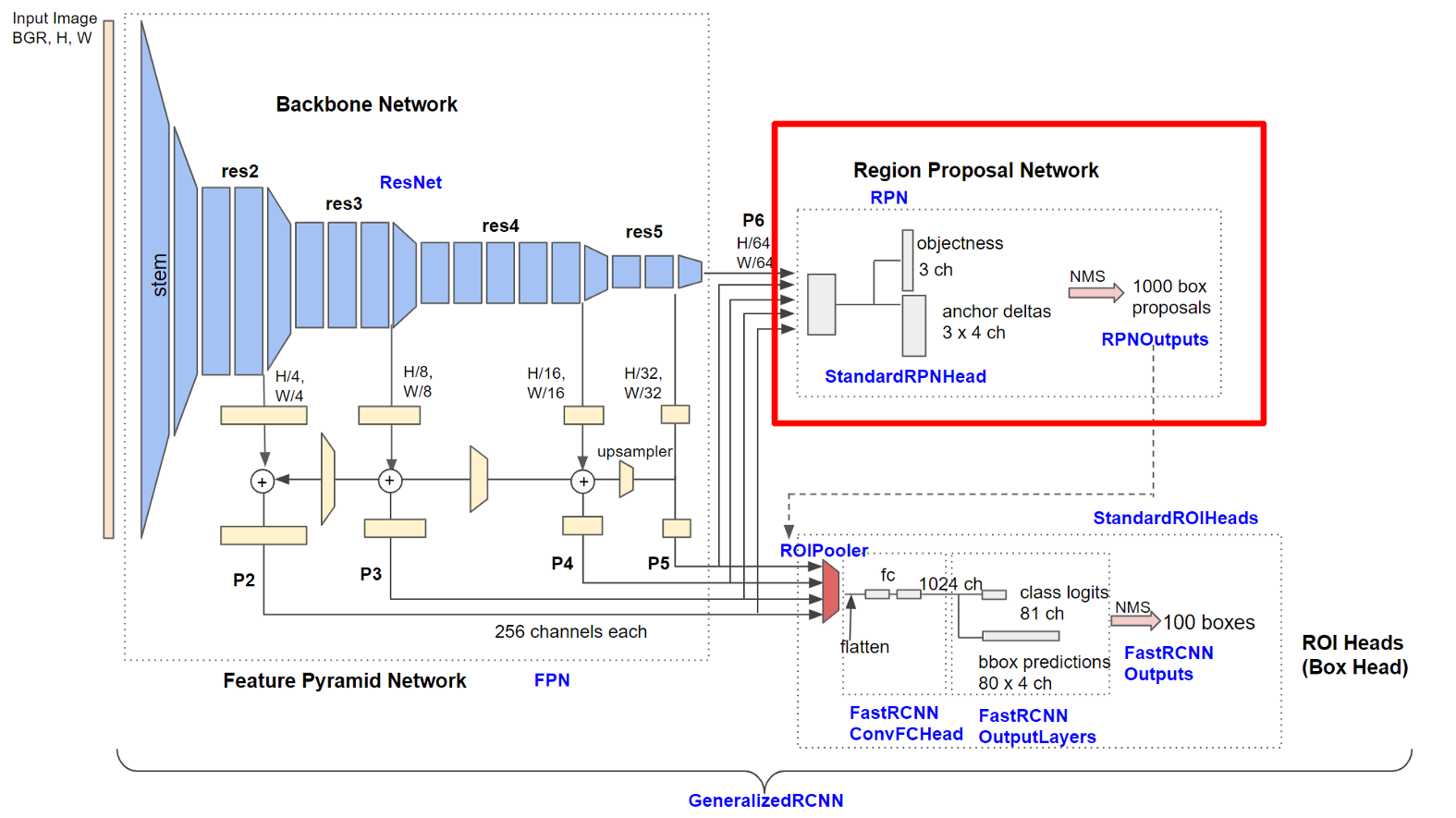
Figure 2. Detailed architecture of Base-RCNN-FPN. Blue labels represent class names.

正如我们在第 2 部分中看到的，特征金字塔网络（Feature Pyramid Network）的输出特征图是：

output[“p2”].shape -> torch.Size([1, 256, 200, 320]) # stride = 4
output[“p3”].shape -> torch.Size([1, 256, 100, 160]) # stride = 8
output[“p4”].shape -> torch.Size([1, 256, 50, 80]) # stride = 16
output[“p5”].shape -> torch.Size([1, 256, 25, 40]) # stride = 32
output[“p6”].shape -> torch.Size([1, 256, 13, 20]) # stride = 64

这也是 RPN 的输入。每个张量大小代表（批次、通道、高度、宽度）。我们在本博客部分中使用上述特征维度。

同时我们也有从数据集里面加载的真实标签值（参考数据加载器和Ground Truth实例）

'gt_boxes': Boxes(tensor([
[100.58, 180.66, 214.78, 283.95],
[180.58, 162.66, 204.78, 180.95]
])),
'gt_classes': tensor([9, 9]) # not used in RPN!

对象检测器（object detectors）如何连接特征图和真实框位置和大小？让我们看看 RPN——RCNN 检测器的核心组件——是如何工作的。

图 3 显示了 RPN 的详细示意图。 RPN 由神经网络（RPN Head）和非神经网络功能组成。在 Detectron 2 中， RPN³ 中的所有计算都 GPU 上执行。

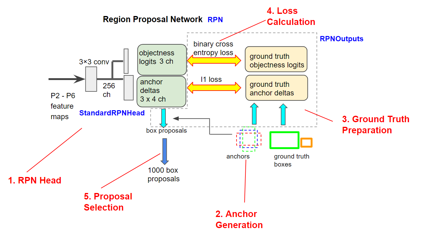
Figure 3. Schematic of Region Proposal Network. Blue and red labels represent class names and chapter titles respectively.

首先，让我们看看RPN head是如何出来来自于FPN的特征图。

1. RPN Head

RPN的神经网络部分很简单。它被称为 RPN Head，由 StandardRPNHHead类中定义的三个卷积层组成。

1. conv (3×3, 256 -> 256 ch)
2. objectness logits conv (1×1, 256 -> 3 ch)
3. anchor deltas conv (1×1, 256 -> 3×4 ch)

五个级别（P2 到 P6）的特征图被一个接一个依次馈送到网络。 每一层的输出两个特征图，如下

1. pred_objectness_logits (B, 3 ch, Hi, Wi): probability map of object existence
2. pred_anchor_deltas (B, 3×4 ch, Hi, Wi): relative box shape to anchors

其中 B 代表批量（batch）大小，Hi 和 Wi 对应于 P2 到 P6 的特征图大小。

他们实际上是什么样子的？在图 4 中，每个级别的 objectness logits map 覆盖在输入图像上。您会发现在 P2 和 P3 处检测到小物体，在 P4 到 P6 处检测到较大的物体。这正是特征金字塔网络的目标。多尺度网络可以检测单尺度检测器无法发现的微小物体。

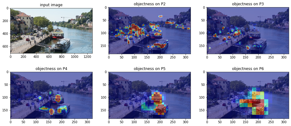
Figure 4. Visualization of objectness maps. Sigmoid function has been applied to the objectness_logits map. The objectness maps for 1:1 anchor are resized to the P2 feature map size and overlaid on the original image.

接下来，让我们接着会讲锚（anchor）的生成，这个是将真实框（ground truth box)与上面的两个输出特征图相关联的必要条件。

1. 锚框生成Anchor Generation

要将对象图（objectness maps）和锚点增量图（anchor deltas map）关联到真实标签框，这就有必要使用称为”锚点（anchor）”的参考框。

2.1 生成锚框

在基础网络架构和代码库结构一节中，锚框被定义成如下形式：

MODEL.ANCHOR_GENERATOR.SIZES = [[32], [64], [128], [256], [512]]
MODEL.ANCHOR_GENERATOR.ASPECT_RATIOS = [[0.5, 1.0, 2.0]]

这是什么意思？
ANCHOR_GENERATOR.SIZES 列表的五个元素对应五个级别的特征图（P2 到 P6）。例如 P2 (stride=4) 有一个大小为 32 的锚点。
纵横比定义了锚的形状。对于上面的示例，共有三种形状：0.5、1.0 和 2.0。让我们看看实际的锚点（图 5）。 P2特征图上的三个anchor的纵横比为1:2、1:1和2:1，面积与32×32相同。在 P3 级锚点是 P2 级锚点的两倍。

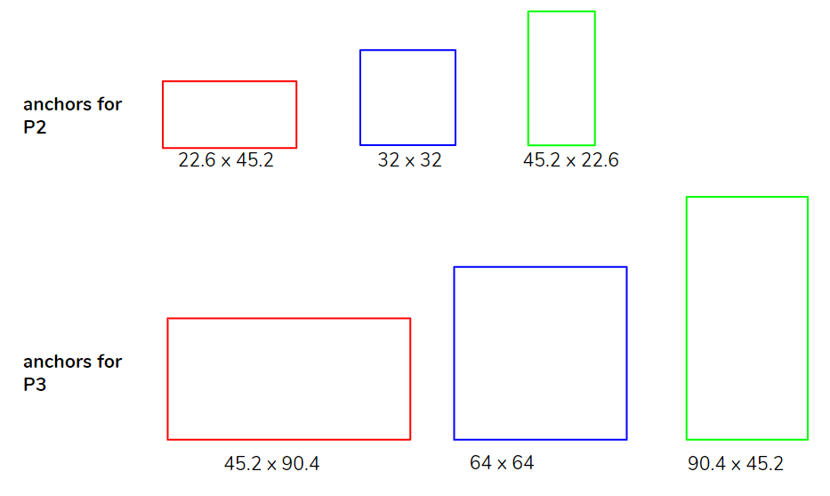
Figure 5. Cell anchors for P2 and P3 feature maps. (from left: 1:2, 1:1 and 2:1 aspect ratios)

这些锚点在 Detectron 2 中称为”单元锚点”。（锚点生成的代码在这里。）因此，我们获得了 5 个特征图级别的 3×5=15 个单元锚点。

cell anchors for P2, P3, P4, P5 and P6. (x1, y1, x2, y2)
tensor([[-22.6274, -11.3137,  22.6274,  11.3137],
        [-16.0000, -16.0000,  16.0000,  16.0000],
        [-11.3137, -22.6274,  11.3137,  22.6274]])
tensor([[-45.2548, -22.6274,  45.2548,  22.6274],
        [-32.0000, -32.0000,  32.0000,  32.0000],
        [-22.6274, -45.2548,  22.6274,  45.2548]])
tensor([[-90.5097, -45.2548,  90.5097,  45.2548],
        [-64.0000, -64.0000,  64.0000,  64.0000],
        [-45.2548, -90.5097,  45.2548,  90.5097]])
tensor([[-181.0193,  -90.5097,  181.0193,   90.5097],
        [-128.0000, -128.0000,  128.0000,  128.0000],
        [ -90.5097, -181.0193,   90.5097,  181.0193]])
tensor([[-362.0387, -181.0193,  362.0387,  181.0193],
        [-256.0000, -256.0000,  256.0000,  256.0000],
        [-181.0193, -362.0387,  181.0193,  362.0387]])

2.2 在网格点上放置锚点

接下来，我们将单元锚点放置在大小与预测特征图相同的网格单元上。

例如，我们预测的特征图”P6″的大小为 (13, 20)，步长为 64。在图 6 中，P6 网格显示为三个锚点位于 (5, 5)。在输入图像分辨率中，(5, 5)的坐标对应于(320, 320)，方形anchor的大小为(512, 512)。锚点放置在每个网格点，因此为 P6 生成了 13×20×3 = 780 个锚点。

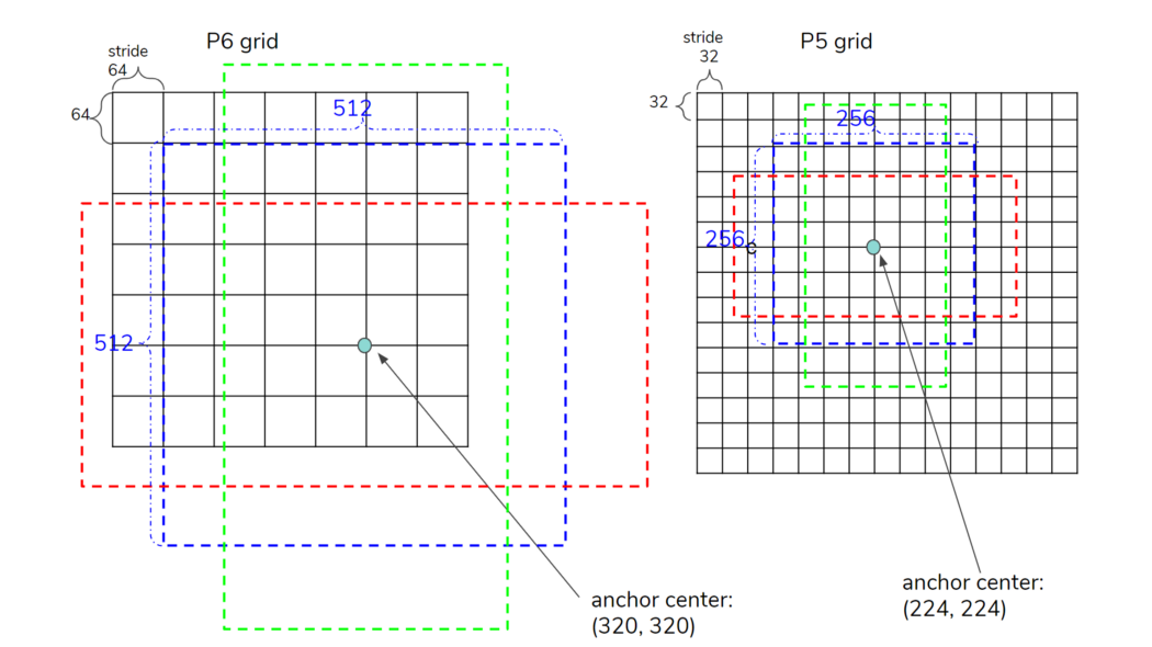
Figure 6. Placing anchors on grid points. The top-left corner of each grid corresponds to (0, 0).

1. Ground Truth 准备

在本章中，我们将标注的真实框与生成的锚点相关联。

3.1 计算教并比（IOU）矩阵

假设我们有两个从数据集中加载的真实 (GT) 框。

'gt_boxes':
Boxes(tensor([
[100.58, 180.66, 214.78, 283.95],
[180.58, 162.66, 204.78, 180.95]
])),

我们现在尝试从255780个anchor中找出与上面两个GT box相似的anchor。如何判断一个box是否与另一个相似？答案是交并比 (IoU) 的计算。在 Detectron2 中，pairwise_iou 函数可以从两个框列表中计算每一对的 IoU。在我们的例子中，pairwise_iou 的结果是一个矩阵，其大小为 (2(GT), 255780(anchors))。

Example of IoU matrix, the result of pairwise_iou
tensor([[0.0000, 0.0000, 0.0000, ..., 0.0000, 0.0000, 0.0000],#GT 1
        [0.0000, 0.0000, 0.0000, ..., 0.0087, 0.0213, 0.0081],#GT 2

3.2 通过Matcher检查IoU 矩阵

所有锚框都被标记为前景、背景或被忽略。如图 7 所示，如果 IoU 大于预定义的阈值（通常为 0.7），则将锚分配给 两个真实（GT） 框之一并标记为前景（’1’）。如果 IoU 小于另一个阈值（通常为 0.3），则锚框被标记为背景（’0’），否则被忽略（’-1’）。

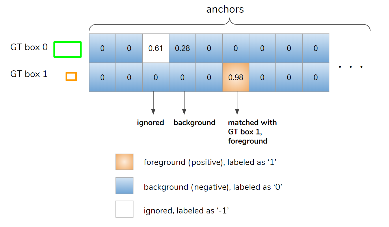
Figure 7. Matcher determines assignment of anchors to ground-truth boxes. The table shows the IoU matrix whose shape is (number of GT boxes, number of anchors).

在图 8 中，我们显示了叠加在输入图像上的匹配结果。如您所见，大多数网格点被标记为背景 (0)，其中一些标记为前景 (1) 和被忽略 (-1)。

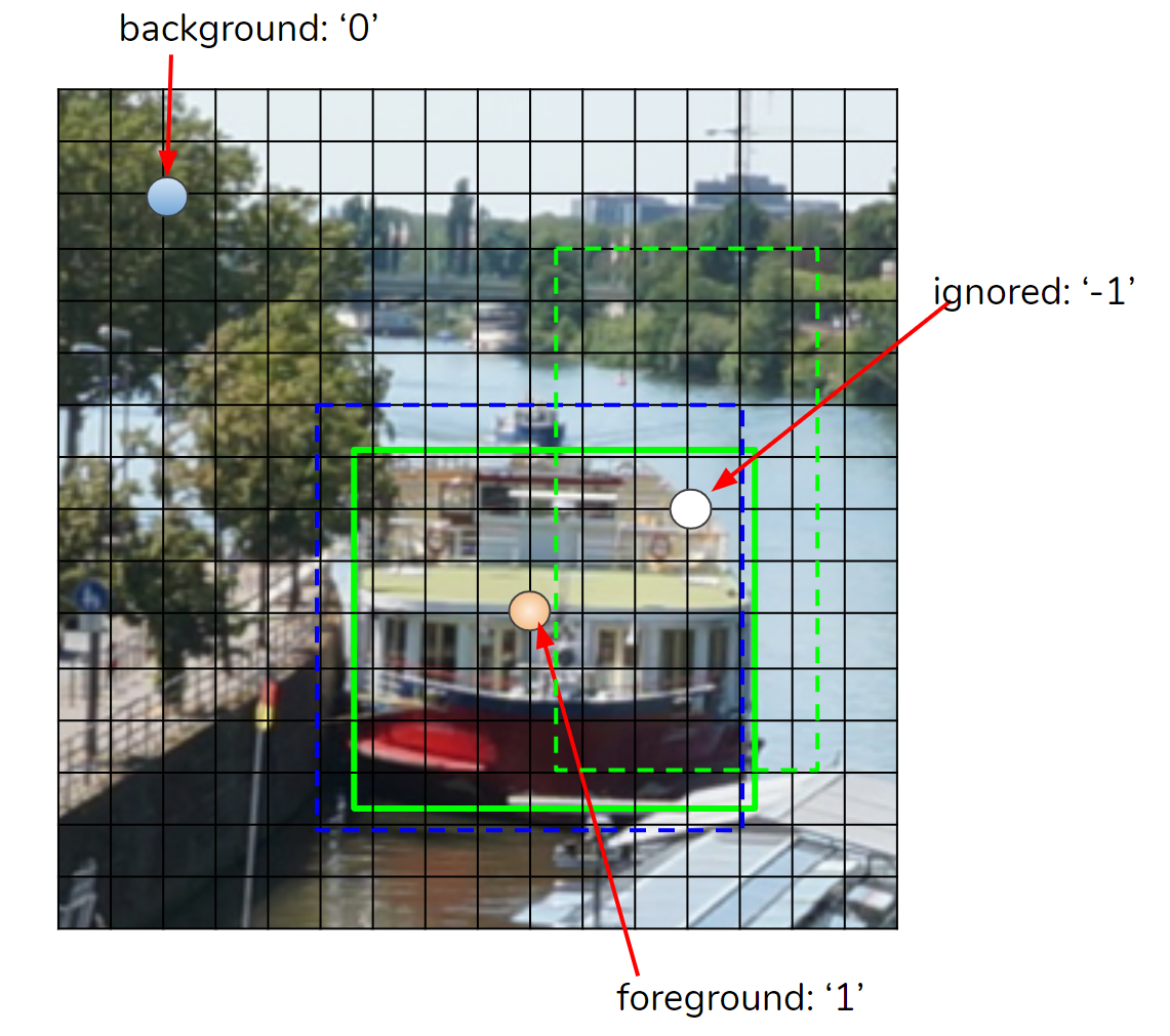
Figure 8. Matching result overlaid on the input image.

3.3 计算锚点增量

确定为前景的锚框与 GT 框具有相似的形状。然而，网络应该学会推理出 GT 盒的确切位置和形状。为了实现它，应该学习四个回归参数：Δx、Δy、Δw 和 Δh。这些”增量”是使用 Box2BoxTransform.get_deltas 函数计算的，如图 9 所示。该公式写在 Faster-RNN paper⁴中。

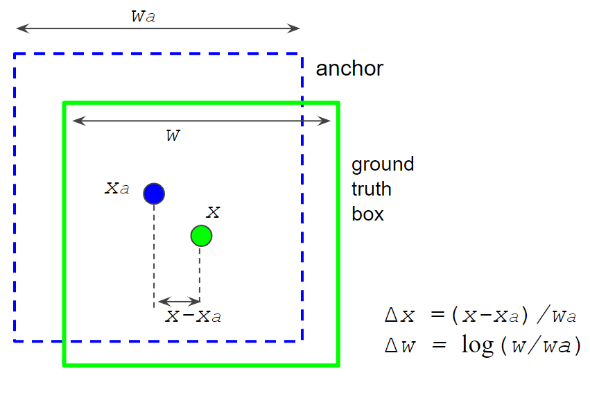
Figure 9. Anchor deltas calculation.

结果，我们获得了一个名为 gt_anchor_deltas 的张量，在我们的例子中它的形状是 (255,780, 4)。

calculated deltas (dx, dy, dw, dh)
tensor([[ 9.9280, 24.6847,  0.8399,  2.8774],
        [14.0403, 17.4548,  1.1865,  2.5308],
        [19.8559, 12.3424,  1.5330,  2.1842],
        ...,

3.4 重新采样框以计算损失

现在我们在特征图的每个网格点上都有 objectness_logits 和 anchor_deltas，我们可以将预测的特征图与它们进行比较。
图 10（左）是每个图像和示例的锚点数量的细分。如您所见，大多数锚点都是背景。例如，通常有少于 100 个前景锚点，在 255,780 个锚点中被忽略的锚点少于 1000 个，其余是背景。如果我们继续训练，由于标签不平衡，很难学习前景的。
使用 subsample_labels 函数重新采样标签以解决不平衡问题。
设 N 为前景 + 背景框的目标数量，F 为前景框的目标数量。 N 和 F/N 由以下配置参数定义。

N: MODEL.RPN.BATCH_SIZE_PER_IMAGE (typically 256)
F/N: MODEL.RPN.POSITIVE_FRACTION (typically 0.5)

图 10（中）显示了重新采样框的细分。随机选择背景和前景框，使 N 和 F/N 成为由上述参数定义的值。如果前景数量小于 F，如图 10（右）所示，背景框被采样以填充 N 个样本。

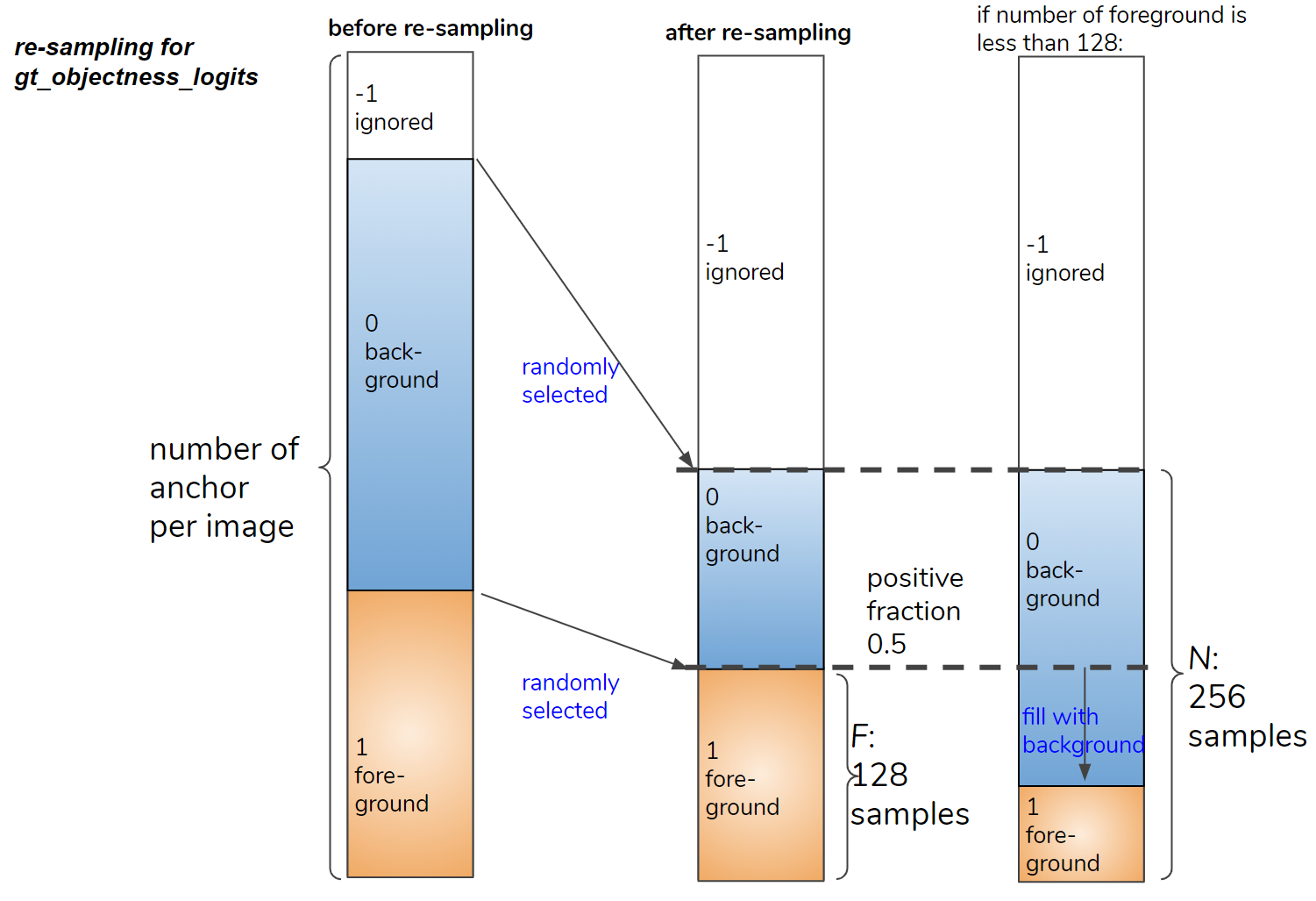
Figure 10. Re-sampling the foreground and background boxes.

1. 损失Loss 计算

两个损失函数应用于 rpn_losses函数的预测和真实特征图（ground truth maps ）。

定位损失（localization loss）

• l1 损失⁵。
• 仅在ground-truth objectness=1（前景）的网格点计算，这意味着忽略所有背景网格点来计算损失。

对象性损失（objectness loss）（objectness loss）

• 二元交叉熵损失。
• 仅在真实对象 = 1（前景）或 0（背景）的网格点处计算。

实际损失结果如下：

{
'loss_rpn_cls': tensor(0.6913, device='cuda:0', grad_fn=<mulbackward0>),
'loss_rpn_loc': tensor(0.1644, device='cuda:0', grad_fn=<mulbackward0>)
}</mulbackward0></mulbackward0>

1. “区域提议”框选择（Proposal Selection）

最后，我们按照以下四个步骤从预测框中选择 1000 个”区域提议”框。

1. 将预测的anchor_deltas应用到对应的anchor上，是3.3的逆过程。
2. 将预测框排序，排序的依据是按对象性（objectness ）预测的得分大小。
3. 如图 11 所示，前 K 个评分框（由配置参数定义）是​​从图像的每个特征级别中选择的image⁶。例如，从 P2 的 192,000 个盒子中选择 2,000 个盒子。对于存在少于 2,000 个框的 P6，将选择所有框。
4. 非最大抑制 (batched_nms) 独立应用于每个级别。结果，1,000 个得分最高的盒子幸存了下来而被选中。

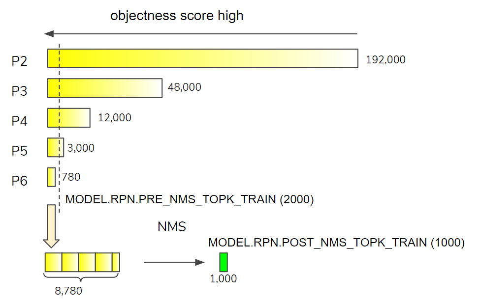
Figure 11. Choosing top-K proposal boxes from each feature level. The numbers of boxes are the examples when input image size is (H=800, W=1280).

在下一部分中，我们将进入 Box head，即 R-CNN 的第二阶段。感谢您的阅读，请等待下一部分！

[1] This is a personal article and the opinions expressed here are my own and not those of my employer.

[2] Yuxin Wu, Alexander Kirillov, Francisco Massa, Wan-Yen Lo and Ross Girshick, Detectron2. GitHub – facebookresearch/detectron2: Detectron2 is FAIR’s next-generation platform for object detection, segmentation and other visual recognition tasks., 2019. The file, directory, and class names are cited from the repository ( Copyright 2019, Facebook, Inc. )
[3] the files used for RPN are: modeling/proposal_generator/rpn.py, modeling/proposal_generator/rpn_outputs.py, modeling/anchor_generator.py, modeling/box_regression.py, modeling/matcher.py and modeling/sampling.py
[4] Shaoqing Ren, Kaiming He, Ross Girshick, and Jian Sun. Faster R-CNN: Towards real-time object detection with region proposal networks. In NIPS, 2015. (link)
[5] Implemented as smooth-l1 loss, but it’s actually pure-l1 loss unlike Detectron1 or MMDetection. (see : link).

[6] In Detectron 1 and maskrcnn-benchmark, the top-K proposals are chosen from a batch during training. (see: link).

Digging into Detectron 2 — part 4 | by Hiroto Honda | Medium

Original: https://blog.csdn.net/zhuguiqin1/article/details/119088420
Author: 程序之巅
Title: 深入理解Detectron 2 — Part 4 区域建议网络（Region Proposal Network）