

S2A-NET
文章目录
基础知识
- 长边13 5 ∘ 135^{\circ}13 5 ∘定义法,a n g l e ∈ [ − 4 5 ∘ , 13 5 ∘ ) angle \in [ -45^{\circ}, 135^{\circ})an g l e ∈[−4 5 ∘,13 5 ∘),t h e t a ∈ [ − π / 4 , 3 ⋅ π / 4 ) theta \in [ -\pi / 4, 3 \cdot \pi / 4)t h e t a ∈[−π/4 ,3 ⋅π/4 )且height> width。
OBB标注方式指任意四边形;顶点按顺时针排序。HBB标注方式指标注示例的外接矩形。
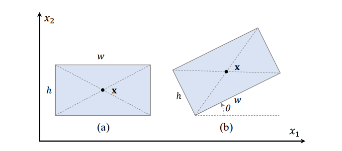
通用的目标检测输出 hbbox(horizontal bounding box)形状,通常表示为{ ( x , w , h ) } { \left( \textbf{x}, w, h\right)}{(x ,w ,h )},其中x = ( x 1 , x 2 ) \textbf{x} = \left(x_{1},x_{2}\right)x =(x 1 ,x 2 )是bbox的中心点坐标。 OBB(oriented bounding box)表示为{ ( x , w , h , θ ) } { \left( \textbf{x}, w, h, \theta \right)}{(x ,w ,h ,θ)},比HBB的表示方式多了一个角度θ \theta θ,在S 2 A − N E T S^{2}A-NET S 2 A −NET论文中,θ ∈ [ − π 4 , 3 π 4 ] \theta \in [ – \frac{\pi}{4}, \frac{3\pi}{4} ]θ∈[−4 π,4 3 π]。当θ = 0 \theta=0 θ=0时,一个OBB就可以看做是一个HBB。在OBB中,w w w和h h h分别表示一个bbox的长边和短边。θ \theta θ是从x 1 x_{1}x 1 位置方向到w w w方向的角度。

; 引言
与基于R-CNN的检测器相比,一阶段的检测器使用规则并且密集的采样anchors回归边界框,并且直接对其进行分类。这种结构具有很高的计算效率,但是往往在精度上不足。
启发式定义的anchors质量较低,无法覆盖物体,导致物体和anchor之间出现错位。这种错位通常会加剧前景背景类的不平衡,并阻碍性能。由于来自backbone网络的卷积特征通常与固定的感受野对齐,然而自然界中的对象以任意方向和不同外观分布。即使一个anchor box以很高的置信度分配给一个实例,但是在anchor box和卷积特征之间仍然存在错位。如下图所示,左边的小图中,红色箭头表示anchor box和卷积特征之间的错位。anchor box是蓝色的框,卷积特征是浅蓝色的框。为了解决这个问题,首先将初始anchor细化为旋转的anchor,如右图中的橙色框框;然后在细化anchor box的引导下,调整特征采样点的位置以提取对齐的深度特征。

网络架构
此论文提出了S 2 A − N e t S^{2}A-Net S 2 A −N e t(Single-shot Alignment Network),由一个backbone网络,一个FPN,和另外两个重要组件FAM(Feature Alignment Module) 和ODM(Oriented Detection Module)组成。FAM和ODM为检测头,应用到特征金字塔的每一层。在FAM中,ARN(Anchor Refinement Network)生成高质量的旋转anchors,然后将这些anchors和输入特征喂入ACL(Alignment Convolution Layer)提取对齐特征。ODM中使用ARF(active rotating filters)生成方向敏感的特征,然后池化特征提取方向不变的特征。最后分类和回归分支生成最后的检测结果。

S 2 A − N e t S^{2}A-Net S 2 A −N e t以RetinaNet作为baseline,RetineNet结构简单,一个backbone网络加上FPN加上分类和回归两个分支子网络。RetineNet中使用Focal loss解决训练过程中的前景和背景不匹配的问题。只不过RetinaNet是为通用目标检测设计的,输出的是HBB形式;S 2 A − N e t S^{2}A-Net S 2 A −N e t输出的是OBB形式,采用长边13 5 ∘ 135^{\circ}13 5 ∘定义法,θ ∈ [ − π 4 , 3 π 4 ] \theta \in [ – \frac{\pi}{4}, \frac{3\pi}{4} ]θ∈[−4 π,4 3 π]。
def forward_train(self, img, img_metas, gt_bboxes, gt_labels, gt_bboxes_ignore=None):
    """Forward function of S2ANet."""
    losses = dict()
    x = self.extract_feat(img)
    outs = self.fam_head(x)

    loss_inputs = outs + (gt_bboxes, gt_labels, img_metas)
    loss_base = self.fam_head.loss(
        *loss_inputs, gt_bboxes_ignore=gt_bboxes_ignore)
    for name, value in loss_base.items():
        losses[f'fam.{name}'] = value

    rois = self.fam_head.refine_bboxes(*outs)

    align_feat = self.align_conv(x, rois)
    outs = self.odm_head(align_feat)

    loss_inputs = outs + (gt_bboxes, gt_labels, img_metas)
    loss_refine = self.odm_head.loss(
        *loss_inputs, gt_bboxes_ignore=gt_bboxes_ignore, rois=rois)
    for name, value in loss_refine.items():
        losses[f'odm.{name}'] = value
    return losses
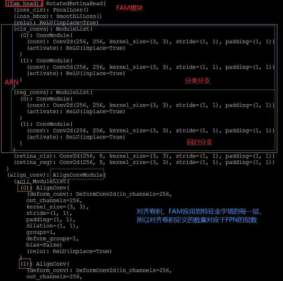
FAM
FAM模块由一个ARN(Anchor Refinement Network)和一个ACL(Alignment Convolution Layer)组成。ARN生成高质量的anchors,ACL利用对齐卷积让特征与相应的anchor进行对齐。
def refine_bboxes(self, cls_scores, bbox_preds):
    """This function will be used in S2ANet, whose num_anchors=1.

    Args:
        cls_scores (list[Tensor]): Box scores for each scale level
            Has shape (N, num_classes, H, W)
        bbox_preds (list[Tensor]): Box energies / deltas for each scale
            level with shape (N, 5, H, W)

    Returns:
        list[list[Tensor]]: refined rbboxes of each level of each image.

"""
    num_levels = len(cls_scores)
    assert num_levels == len(bbox_preds)
    num_imgs = cls_scores[0].size(0)
    for i in range(num_levels):
        assert num_imgs == cls_scores[i].size(0) == bbox_preds[i].size(0)

    device = cls_scores[0].device
    '''
    featmap_sizes list
    [96,128], [48, 64], [24, 32], [12, 16], [6,8]
    '''
    featmap_sizes = [cls_scores[i].shape[-2:] for i in range(num_levels)]
    '''
    mlvl_anchors list
    [12288, 5], [3072, 5], [768, 5], [192, 5], [48, 5]
    '''
    mlvl_anchors = self.anchor_generator.grid_priors(
        featmap_sizes, device=device)

    bboxes_list = [[] for _ in range(num_imgs)]

    for lvl in range(num_levels):
        bbox_pred = bbox_preds[lvl]
        bbox_pred = bbox_pred.permute(0, 2, 3, 1)
        bbox_pred = bbox_pred.reshape(num_imgs, -1, 5)
        anchors = mlvl_anchors[lvl]

        for img_id in range(num_imgs):
            bbox_pred_i = bbox_pred[img_id]
            decode_bbox_i = self.bbox_coder.decode(anchors, bbox_pred_i)
            bboxes_list[img_id].append(decode_bbox_i.detach())

    return bboxes_list
ARN
ARN是两个并行分支组成的轻网络,一个anchor分类分支和一个anchor回归分支。anchor分类分支将anchor按类别进行划分(架构图中省略了此分支),anchor回归分支将水平anchor优化成高质量的旋转anchors。由于我们在对齐卷积中仅仅需要回归anchor box去调整采样位置,在推理阶段,为了加速模型,分类分支被舍弃。
ACL
ACL网络架构中嵌入了对齐卷积。对H × W × 5 H \times W \times 5 H ×W ×5大小的anchor 预测特征图中的每一个位置,首先将它解码成绝对的anchor boxes ( x , w , h , θ ) \left( \textbf{x}, w, h, \theta \right)(x ,w ,h ,θ),然后通过上述公式4计算出offset field,结合输入特征一起喂入对齐卷积提取对齐特征。
每个anchor有五个维度( x , y , w , h , θ ) \left( x,y, w, h, \theta \right)(x ,y ,w ,h ,θ),定期采样九个点获得18维的offset field。每个采样点有两个偏移量(x-offset和y-offset)。

; 对齐卷积
标准的2D卷积中,定义大小为H × W H \times W H ×W的特征图X X X的域为Ω = { 0 , 1 , ⋯ , H − 1 } × { 0 , 1 , ⋯ , W − 1 } \Omega ={0, 1, \cdots, H-1} \times {0,1,\cdots, W-1 }Ω={0 ,1 ,⋯,H −1 }×{0 ,1 ,⋯,W −1 },一个大小为3 × 3 3\times3 3 ×3的窗口定义为R = { ( − 1 , − 1 ) , ( − 1 , 0 ) , ⋯ , ( 0 , 1 ) , ( 1 , 1 ) } R = { \left(-1, -1\right), \left(-1, 0\right),\cdots, \left(0, 1\right),\left(1, 1\right)}R ={(−1 ,−1 ),(−1 ,0 ),⋯,(0 ,1 ),(1 ,1 )},滤波器定义为为W W W,那么输出特征图Y Y Y上的每一位置p ∈ Ω p \in \Omega p ∈Ω计算公式如下:
Y ( p ) = ∑ r ∈ R W ( r ) ⋅ X ( p + r ) ( 1 ) Y\left( p \right) = \sum_{r \in R } W\left( r \right) \cdot X \left( p + r \right) \qquad (1)Y (p )=r ∈R ∑W (r )⋅X (p +r )(1 )
和标准卷积相比,对齐卷积(AlignConv)增添了一个偏移量域O O O,对齐卷积公式如下所示:
Y ( p ) = ∑ r ∈ R ; o ∈ O W ( r ) ⋅ X ( p + r + o ) ( 2 ) Y\left( p \right) = \sum_{r \in R ; o \in O } W\left( r \right) \cdot X \left( p + r + o \right) \qquad (2)Y (p )=r ∈R ;o ∈O ∑W (r )⋅X (p +r +o )(2 )
对于位置p p p,偏移域O O O为基于anchor的采样位置和常规采样位置p + r p+r p +r之间的差异。假设位置p p p相关的anchor为( x , w , h , θ ) \left( \textbf{x}, w, h, \theta \right)(x ,w ,h ,θ),对窗口中的每一个元素r ∈ R r \in R r ∈R,基于anchor的采样位置定义如下:
L p r = 1 S ( x + 1 k ( w , h ) ⋅ r ⋅ R T ( θ ) ) ( 3 ) L_{p}^{r} = \frac{1}{S} \left( x + \frac{1}{k} \left( w, h\right) \cdot r \cdot R^{T}\left( \theta \right)\right) \qquad (3)L p r =S 1 (x +k 1 (w ,h )⋅r ⋅R T (θ))(3 )
其中k k k是滤波器大小,S S S表示特征图的步长,R ( θ ) = ( c o s θ , − s i n θ , s i n θ , c o s θ ) T R\left( \theta \right) = \left( cos\theta, -sin\theta, sin\theta, cos\theta \right)^{T}R (θ)=(cos θ,−s in θ,s in θ,cos θ)T是旋转矩阵,那么位置p p p在偏移域O O O中为:
O = { L p r − p − r } r ∈ R ( 4 ) O = { L_{p}^{r} – p – r }_{r \in R} \qquad (4)O ={L p r −p −r }r ∈R (4 )
通过上述方式,根据相应的anchor box, 就可以将给定位置p p p的卷积特征X ( p ) X\left( p \right)X (p )转换成任意方向的特征卷积特征。与可变性卷积不同的是,对齐卷积的偏移域从anchor中推断出来的。

class AlignConv(nn.Module):
    """Implementation of Align Deep Features for Oriented Object Detection.

    _
"""

    def __init__(self,
                 in_channels,
                 out_channels,
                 kernel_size=3,
                 stride=None,
                 deform_groups=1):
        super(AlignConv, self).__init__()
        self.kernel_size = kernel_size
        self.stride = stride

        self.deform_conv = DeformConv2d(
            in_channels,
            out_channels,
            kernel_size=kernel_size,
            padding=(kernel_size - 1) // 2,
            deform_groups=deform_groups)
        self.relu = nn.ReLU(inplace=True)

    def init_weights(self):
        """Initialize weights of the head."""
        normal_init(self.deform_conv, std=0.01)

    @torch.no_grad()
    def get_offset(self, anchors, featmap_size, stride):
        """Get the offset of AlignConv."""
        dtype, device = anchors.dtype, anchors.device
        feat_h, feat_w = featmap_size
        pad = (self.kernel_size - 1) // 2
        idx = torch.arange(-pad, pad + 1, dtype=dtype, device=device)

        '''
        yy = [[-1, 1, -1], [0, 0, 0], [1, 1, 1]]
        xx = [[-1, 1, -1], [0, 0, 0], [1, 1, 1]]
        '''
        yy, xx = torch.meshgrid(idx, idx)
        xx = xx.reshape(-1)
        yy = yy.reshape(-1)

        xc = torch.arange(0, feat_w, device=device, dtype=dtype)
        yc = torch.arange(0, feat_h, device=device, dtype=dtype)
        yc, xc = torch.meshgrid(yc, xc)
        xc = xc.reshape(-1)
        yc = yc.reshape(-1)
        x_conv = xc[:, None] + xx
        y_conv = yc[:, None] + yy

        x_ctr, y_ctr, w, h, a = torch.unbind(anchors, dim=1)

        x_ctr, y_ctr, w, h = \
            x_ctr / stride, y_ctr / stride, \
            w / stride, h / stride
        cos, sin = torch.cos(a), torch.sin(a)
        dw, dh = w / self.kernel_size, h / self.kernel_size
        x, y = dw[:, None] * xx, dh[:, None] * yy
        xr = cos[:, None] * x - sin[:, None] * y
        yr = sin[:, None] * x + cos[:, None] * y
        x_anchor, y_anchor = xr + x_ctr[:, None], yr + y_ctr[:, None]

        offset_x = x_anchor - x_conv
        offset_y = y_anchor - y_conv

        offset = torch.stack([offset_y, offset_x], dim=-1)
        offset = offset.reshape(anchors.size(0),
                                -1).permute(1, 0).reshape(-1, feat_h, feat_w)
        return offset

    def forward(self, x, anchors):
        """Forward function of AlignConv."""

        anchors = anchors.reshape(x.shape[0], x.shape[2], x.shape[3], 5)

        num_imgs, H, W = anchors.shape[:3]
        offset_list = [
            self.get_offset(anchors[i].reshape(-1, 5), (H, W), self.stride)
            for i in range(num_imgs)
        ]

        offset_tensor = torch.stack(offset_list, dim=0)

        x = self.relu(self.deform_conv(x, offset_tensor.detach()))

        return x
ODM
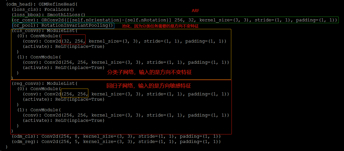
ODM的提出是为了缓解分类分数和定位精度之间的不一致性,从而进行更准确的目标检测。ODM中采用ARF编码方向信息。一个ARF就是一个k × k × N k \times k \times N k ×k ×N滤波器,在卷积过程中主动旋转N − 1 N-1 N −1次,以生成具有N N N个方向通道的特征图(默认情况下,N是8)。对于一个特征图X X X和一个ARF F F F,Y Y Y的第i i i个方向输出可以表示为
Y ( i ) = ∑ n = 0 N − 1 F θ i ( n ) ⋅ X ( n ) , θ i = i 2 π N , i = 0 , ⋯ , N − 1 Y^{\left( i \right)} = \sum_{n=0}^{N-1} F_{\theta_{i}}^{\left( n \right)} \cdot X^{\left( n \right)}, \theta_{i} = i \frac{2\pi}{N}, i=0, \cdots, N-1 Y (i )=n =0 ∑N −1 F θi (n )⋅X (n ),θi =i N 2 π,i =0 ,⋯,N −1
对卷积层应用 ARF可以获得带有特定方向信息编码的方向敏感的特征。bbox回归任务能够从方向敏感特征中获益,但是物体分类任务却需要方向不变特征。通过简单地选择反应最强烈的方向通道作为输出特征X ^ = m a x X ( n ) , 0 < n < N − 1 \hat{X} = max \; X ^{\left( n \right)}, 0 < n < N-1 X ^=ma x X (n ),0 <n <N −1。通过这种方式,我们可以对齐不同方向的对象特征,从而实现鲁棒的对象分类。
对于一个带有8个方向通道大小为H × W × 256 H \times W \times256 H ×W ×256的特征图,池化之后特征图变成H × W × 32 H \times W \times32 H ×W ×32。与方向敏感特征相比,方向不变特征使用更少的参数。最后分别将方向敏感特征和方向不变特征喂入两个子网络回归bbox和分类。
class RotationInvariantPooling(nn.Module):
    """Rotating invariant pooling module."""

    def __init__(self, nInputPlane, nOrientation=8):
        super(RotationInvariantPooling, self).__init__()
        self.nInputPlane = nInputPlane
        self.nOrientation = nOrientation

    def forward(self, x):
        """Forward function."""
        N, c, h, w = x.size()
        x = x.view(N, -1, self.nOrientation, h, w)
        x, _ = x.max(dim=2, keepdim=False)
        return x
class ORConv2d(Conv2d):
    """Oriented 2-D convolution."""
    def __init__(self, in_channels, out_channels, kernel_size=3, arf_config=None, stride=1,
                 padding=0, dilation=1, groups=1, bias=True):
        self.nOrientation, self.nRotation = to_2tuple(arf_config)
        super(ORConv2d, self).__init__(in_channels, out_channels, kernel_size,
                                       stride, padding, dilation, groups, bias)
        self.register_buffer('indices', self.get_indices())
        self.weight = Parameter(
            torch.Tensor(out_channels, in_channels, self.nOrientation, *self.kernel_size))
        if bias:
            self.bias = Parameter(torch.Tensor(out_channels * self.nRotation))

        self.reset_parameters()

    def reset_parameters(self):
        """Reset the parameters of ORConv2d."""
        n = self.in_channels * self.nOrientation
        for k in self.kernel_size:
            n *= k
        self.weight.data.normal_(0, math.sqrt(2.0 / n))
        if self.bias is not None:
            self.bias.data.zero_()

    def get_indices(self):
        """Get the indices of ORConv2d."""
        kernel_indices = {
            1: {
                0: (1, ),
                45: (1, ),
                90: (1, ),
                135: (1, ),
                180: (1, ),
                225: (1, ),
                270: (1, ),
                315: (1, )
            },
            3: {
                0: (1, 2, 3, 4, 5, 6, 7, 8, 9),
                45: (2, 3, 6, 1, 5, 9, 4, 7, 8),
                90: (3, 6, 9, 2, 5, 8, 1, 4, 7),
                135: (6, 9, 8, 3, 5, 7, 2, 1, 4),
                180: (9, 8, 7, 6, 5, 4, 3, 2, 1),
                225: (8, 7, 4, 9, 5, 1, 6, 3, 2),
                270: (7, 4, 1, 8, 5, 2, 9, 6, 3),
                315: (4, 1, 2, 7, 5, 3, 8, 9, 6)
            }
        }
        delta_orientation = 360 / self.nOrientation
        delta_rotation = 360 / self.nRotation
        kH, kW = self.kernel_size
        indices = torch.IntTensor(self.nOrientation * kH * kW, self.nRotation)
        for i in range(0, self.nOrientation):
            for j in range(0, kH * kW):
                for k in range(0, self.nRotation):
                    angle = delta_rotation * k
                    layer = (i + math.floor(
                        angle / delta_orientation)) % self.nOrientation
                    kernel = kernel_indices[kW][angle][j]
                    indices[i * kH * kW + j, k] = int(layer * kH * kW + kernel)
        '''
        indices = [
            [1, 2, 3, 6, 9, 8, 7, 4],
            [2, 3, 6, 9, 8, 7, 4, 1],
            [3, 6, 9, 8, 7, 4, 1, 2],
            [4, 1, 2, 3, 6, 9, 8, 7],
            [5, 5, 5, 5, 5, 5, 5, 5],
            [6, 9, 8, 7, 4, 1, 2, 3],
            [7, 4, 1, 2, 3, 6, 9, 8],
            [8, 7, 4, 1, 2, 3, 6, 9],
            [9, 8, 7, 4, 1, 2, 3, 6],
        ]
        '''
        return indices.view(self.nOrientation, kH, kW, self.nRotation)

    def rotate_arf(self):
        """Build active rotating filter module."""
        return active_rotated_filter(self.weight, self.indices)

    def forward(self, input):
        """Forward function."""

        return F.conv2d(input, self.rotate_arf(), self.bias, self.stride,
                        self.padding, self.dilation, self.groups)
实现
损失函数
假设x g , x , \textbf{x}{g}, \textbf{x},x g ,x ,分别为gt box和anchor box,那么参数化回归目标如下所示:
Δ x g = ( x g − x ) R ( θ ) ⋅ ( 1 w , 1 h ) ( Δ w g , Δ h g ) = l o g ( w g , h g ) − l o g ( w , h ) Δ θ g = 1 π ( θ g − θ + k π ) \begin{matrix} \Delta x{g} = \left( x_{g} – x \right) R\left( \theta \right) \cdot \left( \frac{1}{w}, \frac{1}{h}\right) \ \left( \Delta w_{g} , \Delta h_{g} \right) = log\left( w_{g}, h_{g} \right) – log\left(w, h \right) \ \Delta \theta_{g} = \frac{1}{\pi}\left( \theta_{g} – \theta + k\pi \right) \end{matrix}Δx g =(x g −x )R (θ)⋅(w 1 ,h 1 )(Δw g ,Δh g )=l o g (w g ,h g )−l o g (w ,h )Δθg =π1 (θg −θ+kπ)
其中是一个整数保证。在FAM中,设置表示一个水平anchor,然后回归目标可以表示为上述公式。在ODM中,首先解码FAM的输出,然后通过上述公式重新计算回归目标。
不同于HBB的IoU计算,论文中计算两个OBB之间的IoU。默认情况下,在FAM和ODM中,设置前景的阈值为0.5和背景的阈值为0.4.
S 2 A − N E T S^{2}A-NET S 2 A −NET的损失函数是一个包含FAM和ODM这两部分的多任务损失函数。对于每一部分,我们给每一个anchor/细分anchor一个类别标签并且回归它的位置。论文中采用Focal loss和smooth L1 loss分别作为分类损失函数L c L_{c}L c 和回归损失函数L r L_{r}L r ,那么总的损失函数定义如下:
L = 1 N F ( ∑ i L c ( c i F , l i ∗ ) + ∑ i 1 [ l i ∗ ≥ 1 ] L r ( x i F , g i ∗ ) ) + λ N O ( ∑ i L c ( c i O , l i ∗ ) + ∑ i 1 [ l i ∗ ≥ 1 ] L r ( x i O , g i ∗ ) ) \begin{matrix} L &= \frac{1}{N_{F}} \left( \sum_{i} L_{c} \left( c_{i}^{F} , l_{i}^{} \right) + \sum_{i} 1_{[l_{i}^{} \geq 1]}L_{r} \left( x_{i}^{F}, g_{i}^{}\right)\right) \ &+ \frac{\lambda}{N_{O}} \left( \sum_{i} L_{c} \left( c_{i}^{O} , l_{i}^{} \right) + \sum_{i} 1_{[l_{i}^{} \geq 1]}L_{r} \left( x_{i}^{O}, g_{i}^{}\right)\right) \end{matrix}L =N F 1 (∑i L c (c i F ,l i ∗)+∑i 1 [l i ∗≥1 ]L r (x i F ,g i ∗))+N O λ(∑i L c (c i O ,l i ∗)+∑i 1 [l i ∗≥1 ]L r (x i O ,g i ∗))
其中λ \lambda λ是平衡参数,N F N_{F}N F 和N O N_{O}N O 分别是FAM和ODM中的正样本数量。c i F c_{i}^{F}c i F 和x i F x_{i}^{F}x i F 分别是FAM中的预测类别和anchor i i i的精确位置。c i O c_{i}^{O}c i O 和x i O x_{i}^{O}x i O 分别是ODM中的预测物体类别和bbox的位置。l i ∗ l_{i}^{}l i ∗和g i ∗ g_{i}^{}g i ∗分别是anchor i i i的gt类别和位置。1 [ ⋅ ] 1_{[\cdot]}1 [⋅]是标志函数。
推理
S 2 A − N E T S^{2}A-NET S 2 A −NET是一个全卷积网络。一个输入图像经过bacbone网络提取特征金字塔;紧接着特征金字塔被喂入FAM生成细化的anchor和对齐特征;然后,ODM编码方向信息生成高置信度的预测;最后,选择top-k个预测,并采用NMS生成最后的检测结果。
消融实验
为了验证ARN,ARF和ACL的有效性,论文中做了消融实验。实验结果如下:

; 参考
Original: https://blog.csdn.net/weixin_42111770/article/details/123698494
Author: 陶将
Title: S2A-NET
原创文章受到原创版权保护。转载请注明出处:https://www.johngo689.com/686379/
转载文章受原作者版权保护。转载请注明原作者出处!