数据分析项目实战day2

目录

1.人口数据分析

1.导入并查看相关文件信息

2.进行数据操作

2.政治献金数据分析

1.读取数据查看相关信息

2.进行数据操作

3.用户消费数据分析

1.数据预处理

2.按月进行分析

​ 3.用户个体消费分析

​​​​​​​

1.人口数据分析

1.导入并查看相关文件信息

state表示州的全称，abbreviation表示缩写。

state表示州 areas表示所占面积。

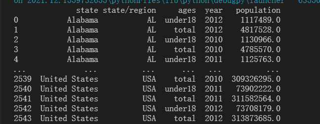
state表示州，age表示调查人口的年龄，year表示统计年份，population表示人口数量。

2.进行数据操作

将人口数据和各州简称数据合并。

上图中有两列缩写，删除其中一列。

将state空值对应的简称找到

对简称进行去重

给为空的state补上正确的值，从而去除nan。

利用之前判别是否存在nan检测操作是否成功。

将面积数据进行合并

找出2010年全部年龄人口数据

完整代码如下：

import numpy as np
import pandas as pd
from pandas.core.indexes.base import Index

abb=pd.read_csv("state-abbrevs.csv")#state表示州全称 abbreviation表示缩写
#print(abb)
area=pd.read_csv("state-areas.csv")#state表示州 areas表示所占面积
#print(area)
pop=pd.read_csv("state-population.csv")#state表示州，age表示调查人口的年龄，year表示统计年份，population表示人口数量。 
#print(pop)
#将人口数据和各州简称数据合并
abb_pop=pd.merge(abb,pop,left_on='abbreviation',right_on='state/region',how='outer')
print(abb_pop.head(5))
abb_pop.drop(labels="abbreviation",axis=1,inplace=True)
print(abb_pop.head(5))

#定位state中nan
abb_pop_nan=abb_pop.loc[abb_pop['state'].isnull()]
abb_pop_statenan=abb_pop_nan['state/region']
#print(abb_pop_statenan)
abb_pop_statenan=abb_pop_statenan.unique()
# print(abb_pop_statenan)

#为空值补上正确的值
#取出USA对应行数据
USA_nan=abb_pop.loc[abb_pop['state/region']=='USA']
PR_nan=abb_pop.loc[abb_pop['state/region']=='PR']
Indexs1=USA_nan.index
Indexs2=PR_nan.index
print(USA_nan)
#获取USA为空对应的行索引并完成赋值
abb_pop.loc[Indexs1,'state']='United States'
abb_pop.loc[Indexs2,'state']='Paraná'
print(abb_pop)

#检测填充nan是否成功
abb_pop_nan=abb_pop.loc[abb_pop['state'].isnull()]
abb_pop_statenan=abb_pop_nan['state/region']
print(abb_pop_statenan)
abb_pop_statenan=abb_pop_statenan.unique()
print(abb_pop_statenan)

#再将面积数据进行合并
abb_pop_area=pd.merge(abb_pop,area,how='outer')
print(abb_pop_area)
#去除面积中含有nan的行
area_nan=abb_pop_area.loc[abb_pop_area['area (sq. mi)'].isnull()]
Indexs3=area_nan.index
abb_pop_area.drop(labels=Indexs3,axis=0,inplace=True)
print(abb_pop_area)

#找出2010年全民数据
total_date_2010=abb_pop_area[abb_pop_area['ages']=='total']
total_date_2010=total_date_2010[total_date_2010['year']==2010]
print(total_date_2010)

#计算各州人口密度 排序并找出人口密度最高
abb_pop_area['density']=abb_pop_area['population']/abb_pop_area['area (sq. mi)']
print(abb_pop_area)
abb_pop_area=abb_pop_area.sort_values(by='density',axis=0,ascending=False)
print(abb_pop_area.head(1))

2.政治献金数据分析

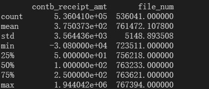
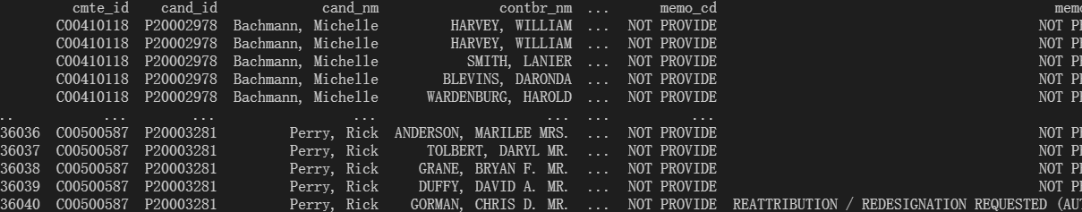
1.读取数据查看相关信息

2.进行数据操作

将所有空值填充为NOT PROVIDE。

将捐赠金额小于等于0的数据删除。

新建一列显示候选人所对应的党派。

统计不同党派出现的次数

统计各个党派收到的献金总数

查看具体每天的献金总数

查看老兵主要支持谁

完整代码如下

import numpy as np
import pandas as pd

parties = {'Bachmann, Michelle': 'Republican',
           'Cain, Herman': 'Republican',
           'Gingrich, Newt': 'Republican',
           'Huntsman, Jon': 'Republican',
           'Johnson, Gary Earl': 'Republican',
           'McCotter, Thaddeus G': 'Republican',
           'Obama, Barack': 'Democrat',
           'Paul, Ron': 'Republican',
           'Pawlenty, Timothy': 'Republican',
           'Perry, Rick': 'Republican',
           "Roemer, Charles E. 'Buddy' III": 'Republican',
           'Romney, Mitt': 'Republican',
           'Santorum, Rick': 'Republican'}

df=pd.read_csv("usa_election.txt")
print(df.head(5))
print(df.info())
print(df.describe())

#将所有空值填充为NOT PROVIDE
df.fillna(value='NOT PROVIDE',inplace=True)
print(df)
#将捐赠金额小于等于0的数据删除
indexs1=df.loc[df['contb_receipt_amt']<=0].index df.drop(labels="indexs1,axis=0,inplace=True)" # print(df) #新建一列显示候选人所对应的党派 df['party']="df['cand_nm'].map(parties)" print(df['party'].value_counts()) #统计各个党派收到的献金总数 party_sum="df.groupby(by='party')['contb_receipt_amt'].sum()" print(party_sum) party_sum_day="df.groupby(by=['party','contb_receipt_dt'])['contb_receipt_amt'].sum()" print(party_sum_day) df_old="df.loc[df['contbr_occupation']=='DISABLED" veteran'] #根据候选人分组 再求和排序 df_old_donate="df_old.groupby(by='cand_nm')['contb_receipt_amt'].sum()" print(df_old_donate.head(1))< code></=0].index>

3.用户消费数据分析

1.数据预处理

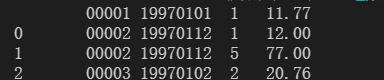
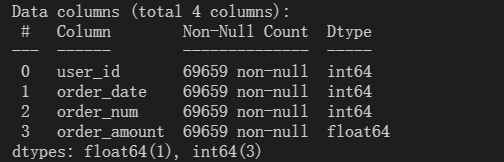
发现数据的列索引存在问题，进行修改。

查看数据信息，发现没有空值。

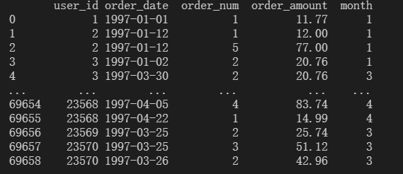
将购买日期转换为时间类型。

在数据新增月份列。

2.按月进行分析

求出每月用户花费的总金额。因为数据跨越了两年，所以不进行刚才的月份合并操作。

绘制折线图。

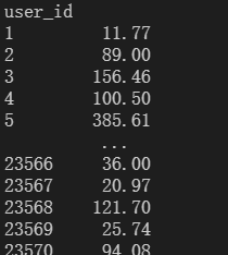
求出每一个用户花费金额。

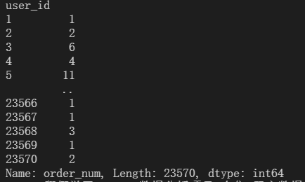
统计每一个用户消费次数。

绘制散点图。

绘制每个用户消费总金额直方图 金额在1200内 。

完整代码如下：

import numpy as np
import pandas as pd
import matplotlib.pyplot as plt

#用以正常显示中文
plt.rcParams['font.sans-serif']=['SimHei'] #用来正常显示中文标签
plt.rcParams['axes.unicode_minus']=False #用来正常显示负号

#修改列索引，name中从左到右依次为用户ID 购买日期 购买数量 购买金额
df=pd.read_csv('CDNOW_master.txt',header=None,sep='\s+',names=['user_id','order_date','order_num','order_amount'])
#print(df)
print(df.info())

#转换时间格式
df['order_date']=pd.to_datetime(df['order_date'],format='%Y%m%d')

#在数据新增月份列
df['month']=df['order_date'].astype('datetime64[M]')
df['month']=[i.month for i in df["month"]]

#统计每个月花费 和购买产品
df_monthly_cost=df.groupby(by='month')['order_amount'].sum()
df_monthly_buy_num=df.groupby(by='month')['order_num'].sum()
print(df_monthly_cost)
print(df_monthly_buy_num)

#作图
plt.figure(figsize=(20,8),dpi=80)
plt.plot(df_monthly_cost,label='每月花费金额')
plt.plot(df_monthly_buy_num,label='每月购买产品数')
plt.legend(loc='best')
plt.show()

#基于用户进行分组
#求每一个用户消费总金额
df_per_user_amount=df.groupby(by='user_id')['order_amount'].sum()
#求每一个用户消费总次数
df_per_user_num=df.groupby(by='user_id').count()['order_num']

print(df_per_user_num)
plt.figure(figsize=(20,8),dpi=80)
plt.scatter(df_per_user_num,df_per_user_amount)
plt.xlabel('购买次数')
plt.ylabel('购买金额')
plt.show()

#绘制每个用户消费总金额直方图 金额在1200内
df_per_user_amount_1=df.groupby(by='user_id').sum().query('order_amount<=1200')["order_amount"] # print(df_per_user_amount_1) plt.figure(figsize="(20,8),dpi=80)" plt.hist(df_per_user_amount_1) plt.xlabel('消费金额') plt.ylabel('用户数量') plt.show() < code></=1200')["order_amount"]>

Original: https://blog.csdn.net/kongqing23/article/details/122337298
Author: kongqing23
Title: 数据分析项目实战day2