

文章目录
*
– 一、pandas的series(一维带标签)
–
+ 1.Series数组的创建
+ 2.series的索引和值
– 二、pandas的DataFrame(二维Series容器)
–
+ 1.pandas读取外部数据
+ 2.DataFrame的创建
+ 3.DataFrame的基础性质
+ 4.DataFrame的索引
+ 5.数据缺失的处理
– 三、pandas的时间序列
–
+ 1.生成一段时间范围
+ 2.DataFrame中使用时间序列
+ 3.pandas重采样
+ 4.举例:
– 四、统计
–
+ 1.练习:统计电影信息(runtime,rating):直方图
+ 2.pandas的统计方法
– 五、数据合并与分组聚合
–
+ 1.练习:统计电影分类情况:条形图
+ 2.数据合并之join
+ 3.数据合并之merge
+ 4.分组聚合
+ 5.索引和复合索引
– 六、练习
–
+ 1.呈现星巴克店铺总数前10的国家
+ 2.呈现中国每个城市的星巴克店铺数量
+ 3.统计不同年份书的数量
+ 4.统计不同年份书的平均评分情况
+ 5.统计911不同类型的紧急情况的次数
+ 6.PM2.5


一、pandas的series(一维带标签)
1.Series数组的创建
① t1 = pd.Series([1,2,15,48,6],index=list("abcde"))
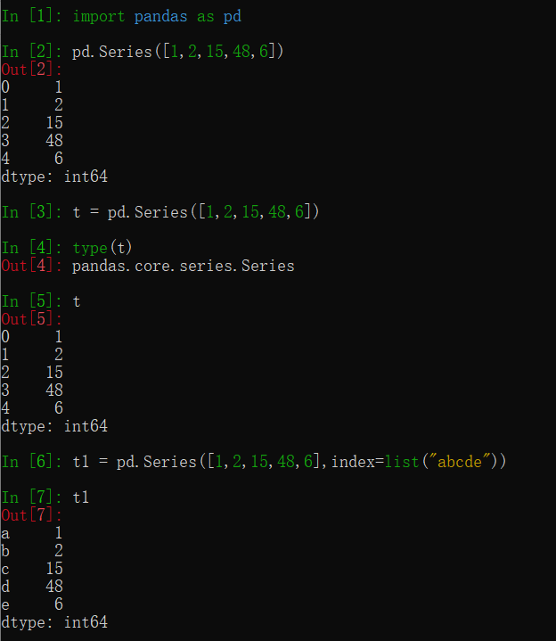
注:其中第一列为所带标签,未指定时默认为索引
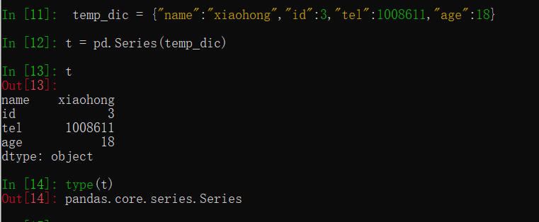
②通过字典创建series,其中索引就是字典中的键
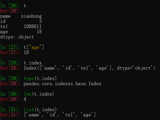
temp_dic = {"name":"xiaohong","id":3,"tel":1008611,"age":18}
t = pd.Series(temp_dic)
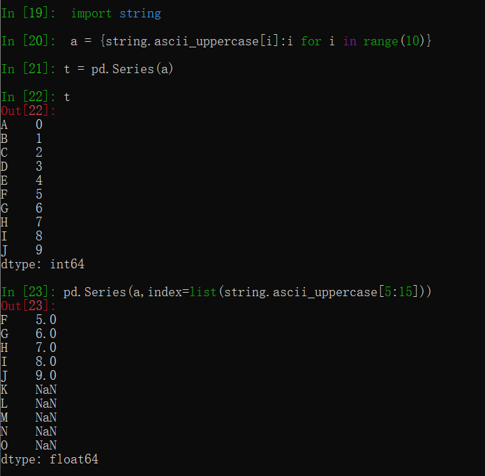
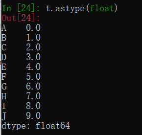
series数组一般必要情况下会自动转换数据类型,其转换数据类型的方法与numpy一样
2.series的索引和值
① t.index
②
t.values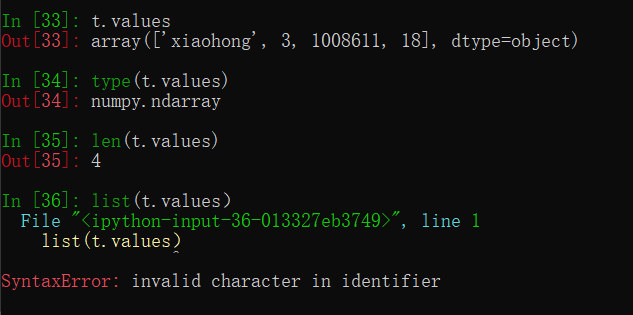
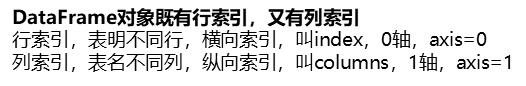
; 二、pandas的DataFrame(二维Series容器)
1.pandas读取外部数据
(1)读取csv中数据
data_csv = "D:\QQ\数据分析课件数据\dogNames2.csv"
df = pd.read_csv(data_csv)
print(df)
(2)读取mysql中数据
pd.read_sql(sql_sentence,connection)
(3)更多读取方法

2.DataFrame的创建
(1)默认索引下
pd.DataFrame(np.arange(12).reshape((3,4)))
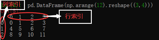
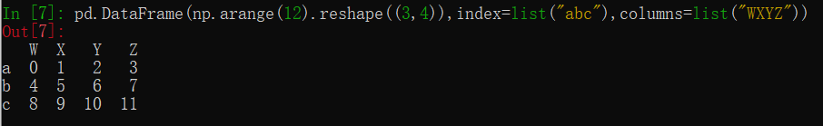
(2)自定义索引
pd.DataFrame(np.arange(12).reshape((3,4)),index=list("abc"),columns=list("WXYZ"))
(3)字典式创建
d1={"name":["xiaohong","xiaoming"],"age":[20,32],"tel":[10086,10045]}
t = pd.DataFrame(d1)
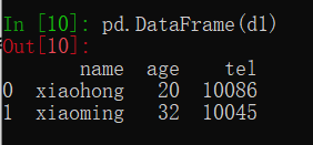
其中字典的键表示DataFrame中的行索引
(4)列表式创建
 d2 = [{"name":"xiaohong","age":"32","tel":10010},{"name":"xiaomin","age":"25","tel":10052},{ "name":"xiaohua","age":15}]
 pd.DataFrame(d2)
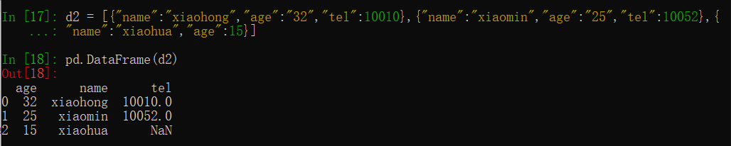
未定义数据时默认NAN
另:DataFrame对象的类型: pandas.core.frame.DataFrame
3.DataFrame的基础性质
print(t.shape)
print(t.dtypes)
print(t.ndim)
print(t.index)
print(t.columns)
print(t.values)
print(t.head(3))
print(t.tail(3))
print(t.info())
print(t.describe())
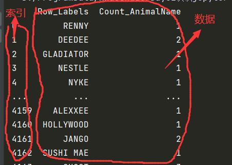
排序方法: df.sort_values(by="Count_AnimalName",ascending=False)
其中:by=表示按照什么排序,ascending=True时表示升序,False表示降序
import pandas as pd
data_csv = "D:\QQ\数据分析课件数据\dogNames2.csv"
df = pd.read_csv(data_csv)

df = df.sort_values(by="Count_AnimalName",ascending=False)

print(df.head())
4.DataFrame的索引
(1)普通索引
pandas去行或列索引的注意点:
1.方括号写数组,表示取行,对行进行操作
2.写字符串,表示的取列索引,对列索引进行操作
print(df[:20])
print(df["Row_Labels"])
print(type(df["Row_Labels"]))

print(df[:20]["Row_Labels"])
(2)经过pandas优化过选择方式:
前景:
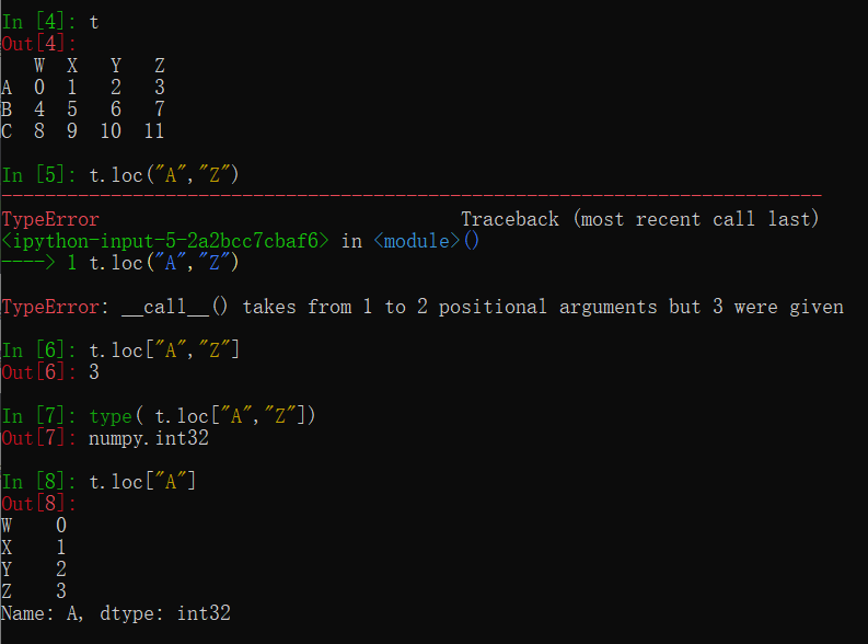
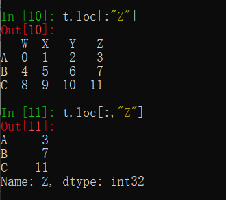
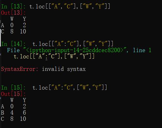
因为普通索引用字符串表示取列索引,而有些行索引也为字符串,这时就需要loc[“A”]表示取行索引为”A”的数据
1.df.loc通过标签索引行数据
t.loc["A","Z"]
2.df.iloc通过位置获取行数据
t.iloc[1]
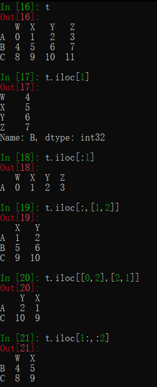
赋值:
t.iloc[1:,:2]=12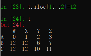
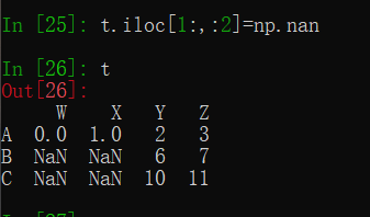
其中转换为nan时自动转型
(3)pandas之布尔索引
索引为bool类型:True,False
print(df[df["Count_AnimalName"]>50])
print(df[(df["Count_AnimalName"]>50)&(df["Count_AnimalName"]<80)])
print(df[(df["Count_AnimalName"]>90)|(df["Count_AnimalName"]<2)])

print(df[(df["Count_AnimalName"]>50)&(df["Row_Labels"].str.len()>4)])
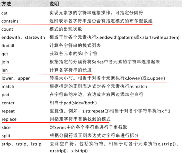
另:pandas字符串方法:
如: df["Row_Labels"].str.len()
5.数据缺失的处理
数据缺失:
1.None,在pandas下是NaN和(np.nan)一样
2.让其为0(有时有意义,不为缺失数据)
缺失数据的处理:
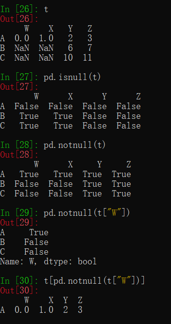
1.NaN数据:先判断是否有NaN:pd.isnull(df),pd.notnull(df)
pd.isnull(t)
pd.notnull(t)
pd.notnull(t["W"])
 t[pd.notnull(t["W"])]
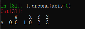
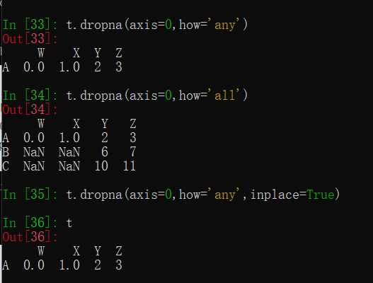
处理方式1:删除NaN所在行列dropna(axis=0,how=’any’,inplace=False)
其中{ axis=0表示按轴为0处理,how=’any’表示只要该行有nan就删除,而how=’all’表示全为nan时才删除,inplace=True表示原地替换相当于赋值给自己df }
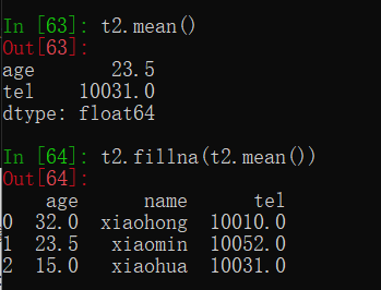
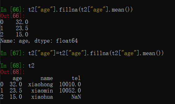
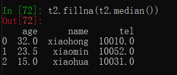
处理方式2:填充数据,t.fillna(t.mean()),t.fillna(t.median()),t.fillna(0)
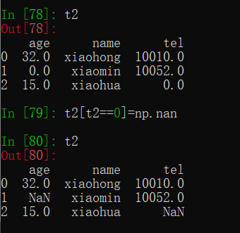
2.处理为0的数据:t[t==0]=np.nan ,再按nan数据类型处理缺失数据
原因:计算平均值时,nan是不参与计算的,但是0会
三、pandas的时间序列
1.生成一段时间范围

其中
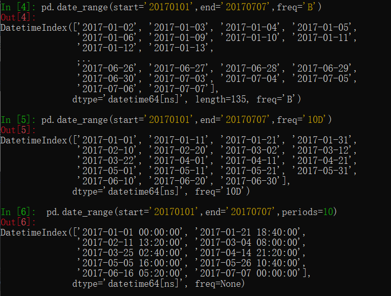
start=表示起始日期, end=表示末位日期, periods=表示时间索引的个数, freq=表示时间索引的频率,该方法的返回值是一个时间索引
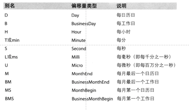
关于频率的更多缩写:(可以使用:10D)
 pd.date_range(start='20170101',end='20170707',freq='10D')
 pd.date_range(start='20170101',end='20170707',periods=10)
2.DataFrame中使用时间序列
(1)

(2)
period = pd.PeriodIndex(year=df["year"],month=df["month"],day=df["day"],hour=df["hour"],freq="H")
该方法可以将多个零散的数据整合成一个时间序列
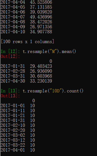
3.pandas重采样


t.resample("M").mean()
 t.resample("10D").count()
4.举例:
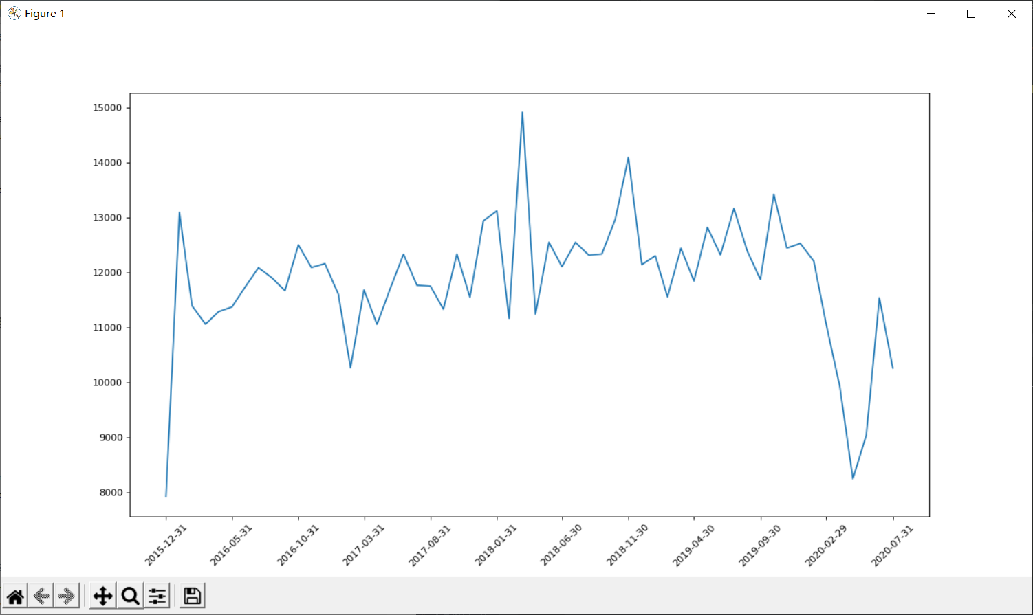
(1)统计911不同月份电话次数的变化情况
import numpy as np
import pandas as pd
from matplotlib import pylab as p
from matplotlib import font_manager
my_font = font_manager.FontProperties(fname="C:\Windows\Fonts\simkai.ttf")

file_path = "D:\ProgramData\课件数据\datasourse\911\911.csv"
df = pd.read_csv(file_path)

df["timeStamp"] = pd.to_datetime(df["timeStamp"])

df.set_index("timeStamp",inplace=True)

count_by_month = df.resample("M").count()["title"]

p.figure(figsize=(15,8),dpi=80)

x = count_by_month.index
y = count_by_month.values
p.plot(x,y)

p.xticks(x[::5],rotation=45)

p.show()
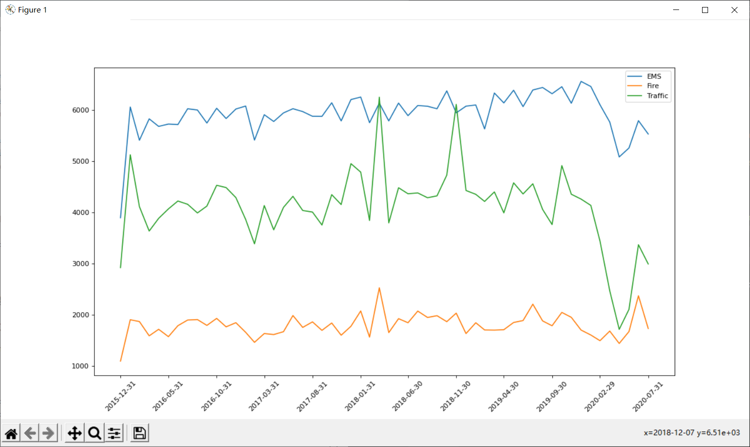
(2)
import numpy as np
import pandas as pd
from matplotlib import pylab as p
from matplotlib import font_manager
my_font = font_manager.FontProperties(fname="C:\Windows\Fonts\simkai.ttf")

file_path = "D:\ProgramData\课件数据\datasourse\911\911.csv"
df = pd.read_csv(file_path)

df["timeStamp"] = pd.to_datetime(df["timeStamp"])

temp_list = df["title"].str.split(":").tolist()
type_list = [i[0] for i in temp_list]
df["type"] = pd.DataFrame(np.array(type_list).reshape((df.shape[0],1)))

df.set_index("timeStamp",inplace=True)

p.figure(figsize=(15, 8), dpi=80)

for group_name,group_data in df.groupby(by="type"):

    count_by_month = group_data.resample("M").count()["title"]

    x = count_by_month.index
    y = count_by_month.values
    p.plot(x, y, label=group_name)

p.xticks(x[::5], rotation=45)

p.legend(loc="best")
p.show()
四、统计
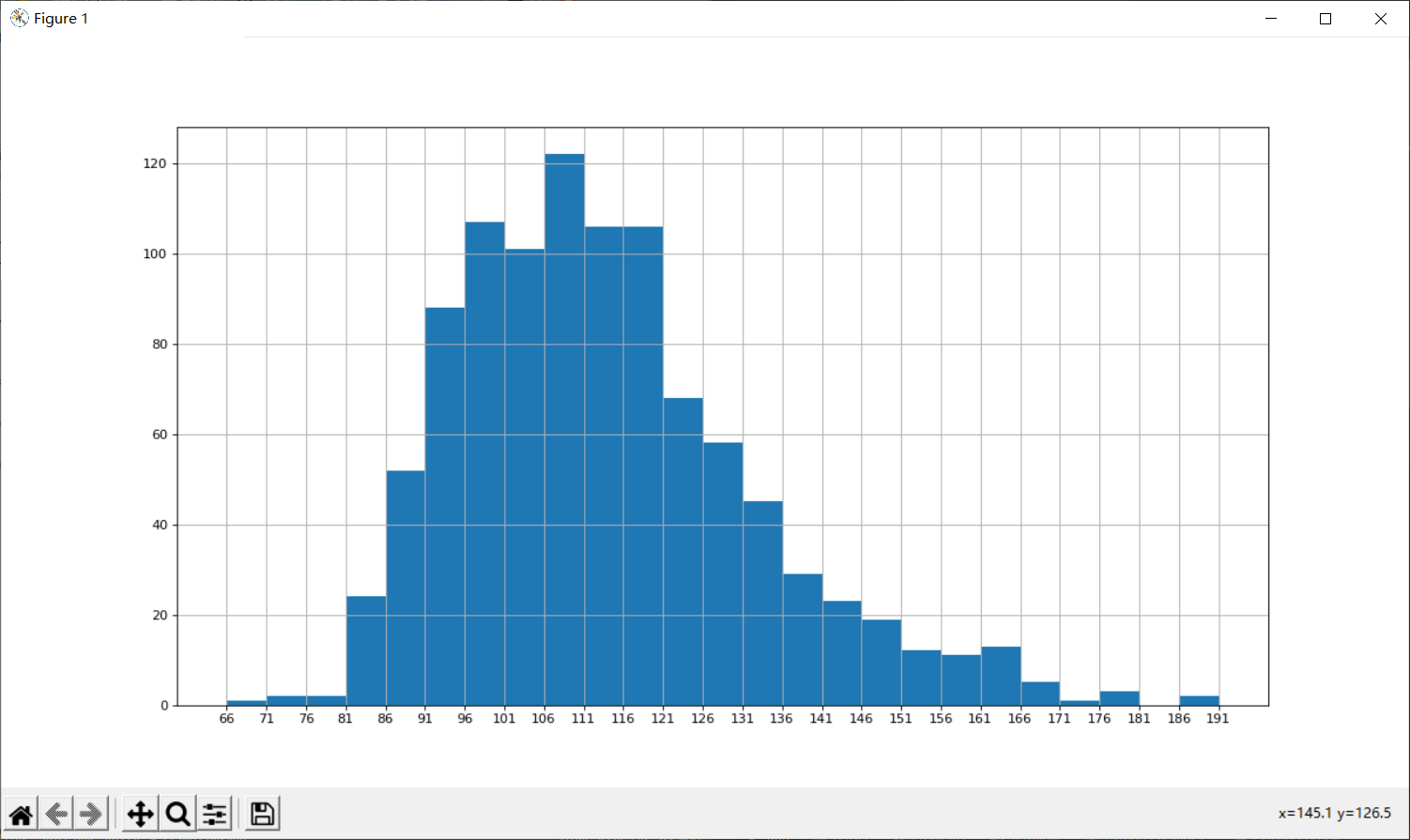
1.练习:统计电影信息(runtime,rating):直方图
(1)runtime
import pandas as pd
from matplotlib import pyplot as p

file_path = "D:\ProgramData\课件数据\datasets_IMDB-Movie-Data.csv"
df = pd.read_csv(file_path)

runtime_data = df["Runtime (Minutes)"].values
t2 = df["Rating"].tolist()

max_runtime = runtime_data.max()
min_runtime = runtime_data.min()

num_bin = (max_runtime-min_runtime)//5

p.figure(figsize=(15,8),dpi=80)

p.hist(runtime_data,num_bin)

p.xticks(range(min_runtime,max_runtime+5,5))

p.grid()

p.show()
(2)rating
import pandas as pd
from matplotlib import pyplot as p

file_path = "D:\ProgramData\课件数据\datasets_IMDB-Movie-Data.csv"
df = pd.read_csv(file_path)

rating_data = df["Rating"].values

max_rating = rating_data.max()
min_rating = rating_data.min()

num_bin_list = [1.6,3.6]
i = num_bin_list[1]
while imax_rating+0.5:
    i=i+0.5
    num_bin_list.append(i)

p.figure(figsize=(15,8),dpi=80)

p.hist(rating_data,num_bin_list)

p.xticks(num_bin_list)

p.grid()

p.show()
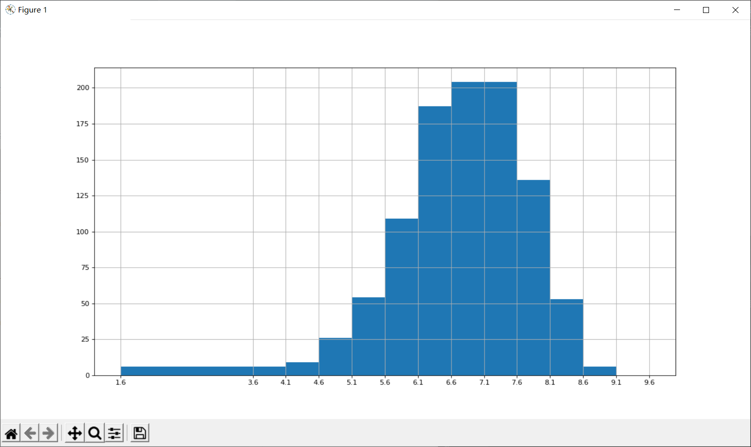
另:还有部分问题尚未解决
2.pandas的统计方法
print(df["Rating"].mean())
print(len(df["Director"].unique()))
temp_actors_list = df["Actors"].str.split(",").tolist()
actors_list = [i for j in temp_actors_list for i in j]
actors_num = len(set(actors_list))
print(actors_num)
max_runtime = df["Runtime (Minutes)"].max()
max_runtime_index = df["Runtime (Minutes)"].argmax()
min_runtime = df["Runtime (Minutes)"].min()
mina_runtime_index = df["Runtime (Minutes)"].argmin()
runtime_median = df["Runtime (Minutes)"].median()
五、数据合并与分组聚合
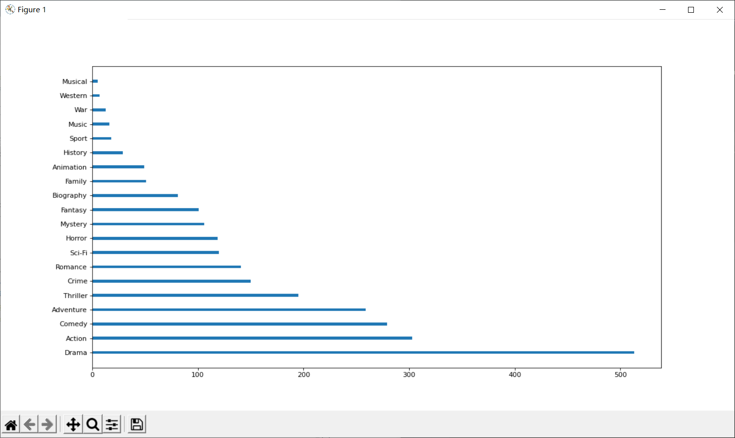
1.练习:统计电影分类情况:条形图
字符串离散:
思路:重新构造一个全为0的数组,列名为分类,如果某一条数据中分类出现过,就让0变为1
import numpy as np
import pandas as pd
from matplotlib import pylab as p

"""
统计电影分类情况
思路:重新构造一个全为0的数组,列名为分类,如果某一条数据中分类出现过,就让0变为1
"""
file_path = "D:\ProgramData\课件数据\datasets_IMDB-Movie-Data.csv"
df = pd.read_csv(file_path)

temp_list = df["Genre"].str.split(",").tolist()

genre_list = list(set([i for j in temp_list for i in j]))

zero_df = pd.DataFrame(np.zeros((df.shape[0],len(genre_list))),columns=genre_list)

for i in range(df.shape[0]):
    zero_df.loc[i,temp_list[i]]=1

genre_count = zero_df.sum(axis=0)

genre_count = genre_count.sort_values(ascending=False)

_x = genre_count.values
_y = genre_count.index

p.figure(figsize=(15,8),dpi=80)
p.barh(range(len(_y)),_x,height=0.2)
p.yticks(range(len(_y)),_y)

p.show()
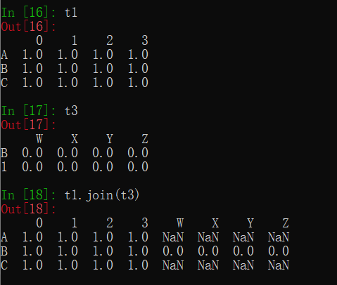
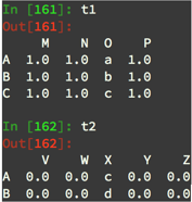
2.数据合并之join
join:默认情况下是把 行索引相同的数据合并在一起

t1.join(t2)
注意:
1.若index(t1)>index(t2),用NaN补充t2少的那一行
2.若index(t1)
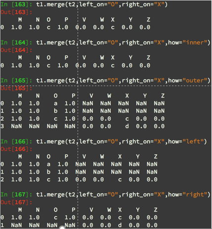
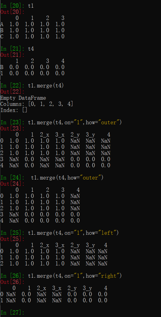
3.数据合并之merge

t1.merge(t4,left_on="a",right_on="c",how="outer")
t1.merge(t4,on="1",how="left")
注意:
(1).其中” on="1"“表示在某一列索引上处理数据,不存在相同索引的可以用” left_on="a",right_on="c" “表示左边列索引为a的与右边列索引为c的看作相同索引,进行处理
(2).其中” how="left"“表示合并方式,默认情况下为 how="inner"表示交集, how="outer"表示并集NaN补全, how="left"表示左边为准NaN补全, how="right"表示右边为准NaN补全
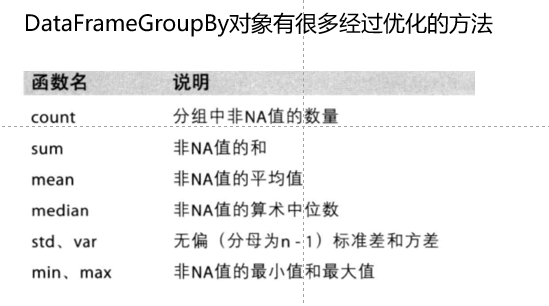
4.分组聚合
pandas中类似的分组的操作: df.groupby(by="columns_name")

DataFrameGroupBy对象:1.可以遍历 2.可以调用聚合方法
for i,j in grouped:
    print(i)
    print("-"*100)
    print(j)
    print("*"*100)

country_count = grouped["Brand"].count()

print(country_count["US"])
print(country_count["CN"])
举例:统计中国每个省份星巴克的数量
china_data = df[df["Country"]=="CN"]

grouped = china_data.groupby(by="State/Province")["Brand"].count()
(1)数据按照多个条件进行分组,返回Series类型
grouped1 = df["Brand"].groupby(by=[df["Country"],df["State/Province"]]).count()
grouped2 = df.groupby(by=["Country","State/Province"]).count()
(2)数据按照多个条件进行分组,返回DataFrame类型
grouped1 = df[["Brand"]].groupby(by=[df["Country"],df["State/Province"]]).count()
grouped2 = df.groupby(by=[df["Country"],df["State/Province"]]).count()[["Brand"]]
grouped3 = df.groupby(by=[df["Country"],df["State/Province"]])[["Brand"]].count()
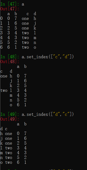
5.索引和复合索引
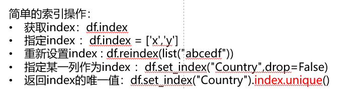
(1)获取index(2)指定index
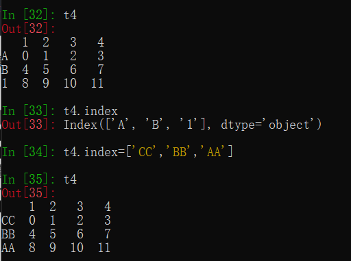
(3)
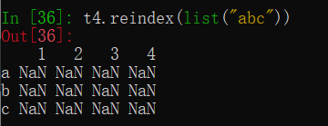
t4.reindex(list("abc"))
相当于在原数组t4中取index为”abc”的数据,若不存在就为NaN
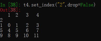
(4)指定某一列作为该数组的index
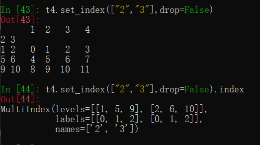
t4.set_index("2",drop=False)

t4.set_index(["2","3"],drop=False)
指定某一列作为该数组的index,其中drop=False表示保留所取列
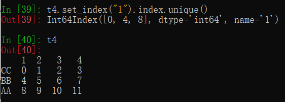
(5)返回index的唯一值
t4.set_index("1").index.unique()
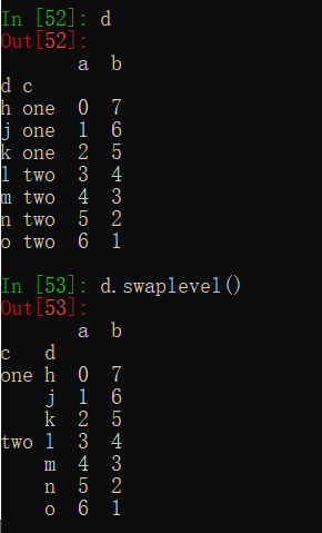
(6)交换内外列表
d.swaplevel()
六、练习
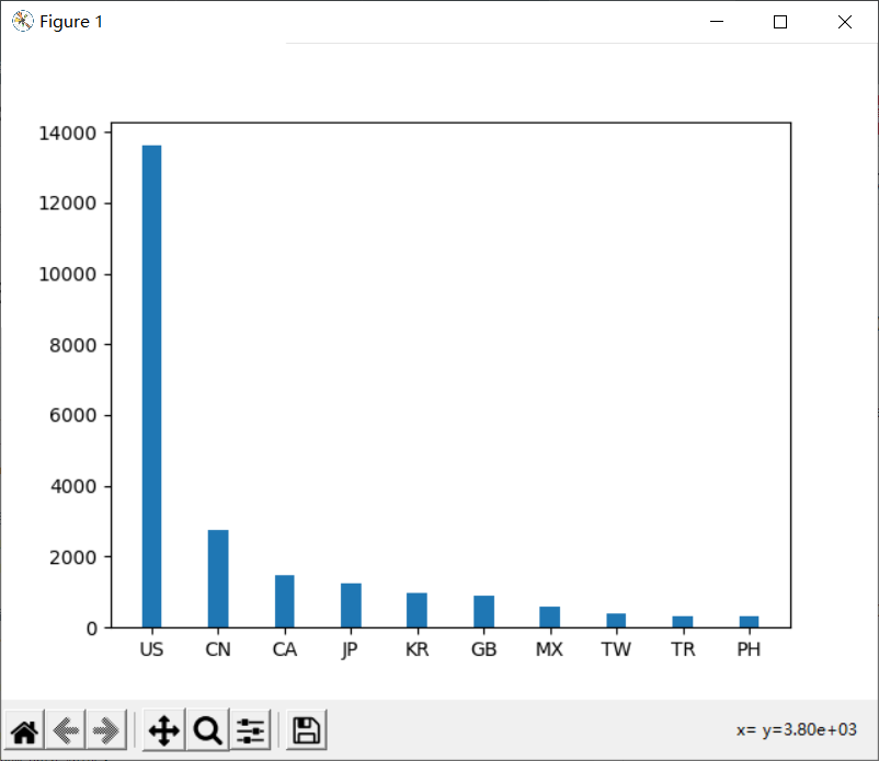
1.呈现星巴克店铺总数前10的国家
import pandas as pd
from matplotlib import pylab as p

file_path = "D:\ProgramData\课件数据\datasourse\星巴克\directory.csv"
df = pd.read_csv(file_path)

num_data = df.groupby(by="Country").count()["Brand"].sort_values(ascending=False)[:10]

_x = num_data.index
_y = num_data.values

p.bar(range(len(_x)),_y,width=0.3)

p.xticks(range(len(_x)),_x)

p.show()
2.呈现中国每个城市的星巴克店铺数量
import pandas as pd
from matplotlib import pylab as p
from matplotlib import font_manager

my_font = font_manager.FontProperties(fname="C:\Windows\Fonts\simkai.ttf")

file_path = "D:\ProgramData\课件数据\datasourse\星巴克\directory.csv"
df = pd.read_csv(file_path)

data = df.groupby(by=["Country","City"])["Brand"].count()
num_data = data["CN"].sort_values(ascending=False)[:40]

_x = num_data.values
_y = num_data.index

p.figure(figsize=(15,10),dpi=80)

p.barh(range(len(_y)),_x,height=0.4)

p.yticks(range(len(_y)),_y,fontproperties=my_font)

p.grid()

p.show()

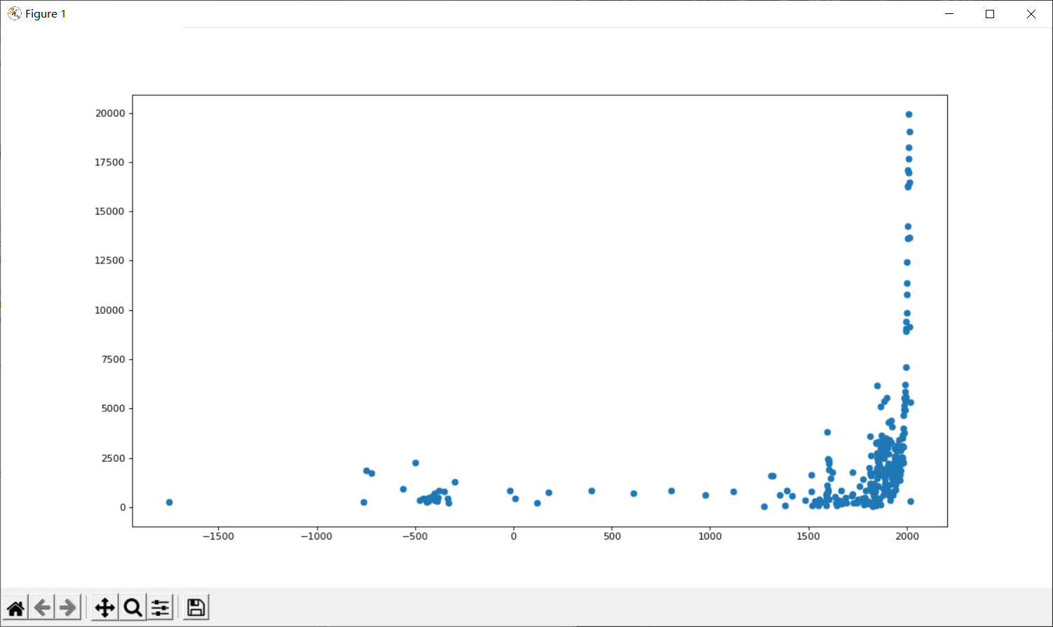
3.统计不同年份书的数量
import pandas as pd
from matplotlib import pylab as p
from matplotlib import font_manager
my_font = font_manager.FontProperties(fname="C:\Windows\Fonts\simkai.ttf")

file_path = "D:/ProgramData/课件数据/datasourse/10000本书/books.csv"
df = pd.read_csv(file_path)

data = df["books_count"].groupby(by=df["original_publication_year"]).sum().sort_values(ascending=False)

x = data.index
y = data.values

p.figure(figsize=(15,8),dpi=80)

p.scatter(x,y)

p.show()
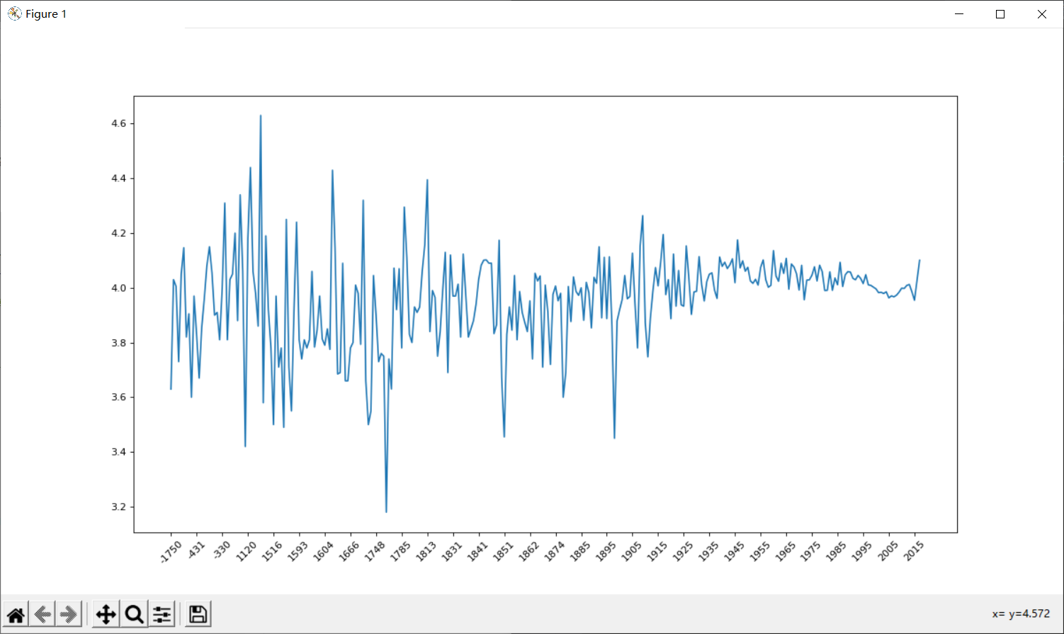
4.统计不同年份书的平均评分情况
import pandas as pd
from matplotlib import pylab as p
from matplotlib import font_manager
my_font = font_manager.FontProperties(fname="C:\Windows\Fonts\simkai.ttf")

file_path = "D:/ProgramData/课件数据/datasourse/10000本书/books.csv"
df = pd.read_csv(file_path)

data = df.groupby(by="original_publication_year")["average_rating"].mean()

_x = data.index
_y = data.values

p.figure(figsize=(15,8),dpi=80)

p.plot(range(len(_x)),_y)

p.xticks(list(range(len(_x)))[::10],_x[::10].astype(int),rotation=45)

p.show()
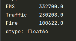
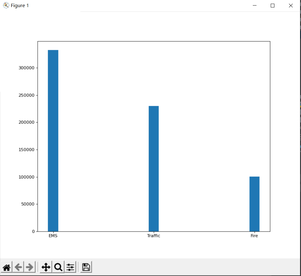
5.统计911不同类型的紧急情况的次数
import numpy as np
import pandas as pd
from matplotlib import pylab as p
from matplotlib import font_manager
my_font = font_manager.FontProperties(fname="C:\Windows\Fonts\simkai.ttf")

file_path = "D:\ProgramData\课件数据\datasourse\911\911.csv"
df = pd.read_csv(file_path)

temp_list = df["title"].str.split(":").tolist()
data_list = list(set([i[0] for i in temp_list]))

zero_df = pd.DataFrame(np.zeros((df.shape[0],len(data_list))),columns=data_list)

for i in data_list:
    zero_df[i][df["title"].str.contains(i)]=1

type_count = zero_df.sum(axis=0)
print(type_count)

_x = type_count.index
_y = type_count.values

p.figure(figsize=(15,8),dpi=80)

p.bar(_x,_y,width=0.1)

p.show()
6.PM2.5
import pandas as pd
import pylab as p

file_path = "D:\ProgramData\课件数据\datasourse\城市空气质量数据\BeijingPM20100101_20151231.csv"
df = pd.read_csv(file_path)

period = pd.PeriodIndex(year=df["year"],month=df["month"],day=df["day"],hour=df["hour"],freq="H")

df["datetime"] = period

df.set_index("datetime",inplace=True)

df = df.resample("10D").mean()

data = df["PM_US Post"].dropna()
data_chain = df["PM_Dongsi"].dropna()

x=data.index
x=[i.strftime("%Y%m%d") for i in x]
x_chain = [i.strftime("%Y%m%d") for i in data_chain.index]
y=data.values
y_chain = data_chain.values

p.figure(figsize=(15,8),dpi=80)
p.plot(range(len(x)),y,label="US")
p.plot(range(len(x_chain)),y_chain,label="CN")
p.xticks(range(0,len(x),10),list(x)[::10],rotation=45)

p.legend()
p.show()
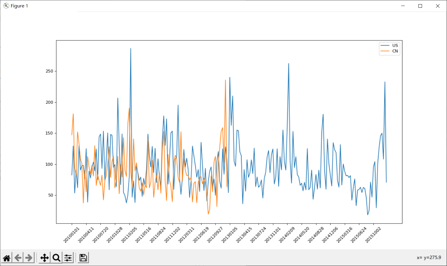
注意:该图像橙色后半部分缺失原因与该数据在该段时间内缺失有关
Original: https://blog.csdn.net/XST1520203418/article/details/119237688
Author: 秋酿玖心
Title: pandas及与matplotlib结合
原创文章受到原创版权保护。转载请注明出处:https://www.johngo689.com/677651/
转载文章受原作者版权保护。转载请注明原作者出处!