

所有的数据来源:链接:https://pan.baidu.com/s/1vTaw1n77xPPfKk23KEKARA
提取码:5gl2
1 Support Vector Machines
1.1 Prepare datasets
import numpy as np
import pandas as pd
import matplotlib.pyplot as plt
import seaborn as sb
from scipy.io import loadmat
from sklearn import svm

'''
1.Prepare datasets
'''
mat = loadmat('data/ex6data1.mat')
print(mat.keys())

X = mat['X']
y = mat['y']
'''大多数SVM的库会自动帮你添加额外的特征x0,所以无需手动添加。'''
def plotData(X, y):
    plt.figure(figsize=(8, 6))
    plt.scatter(X[:, 0], X[:, 1], c=y.flatten(), cmap='rainbow')

    plt.xlabel('x1')
    plt.ylabel('x2')

    pass
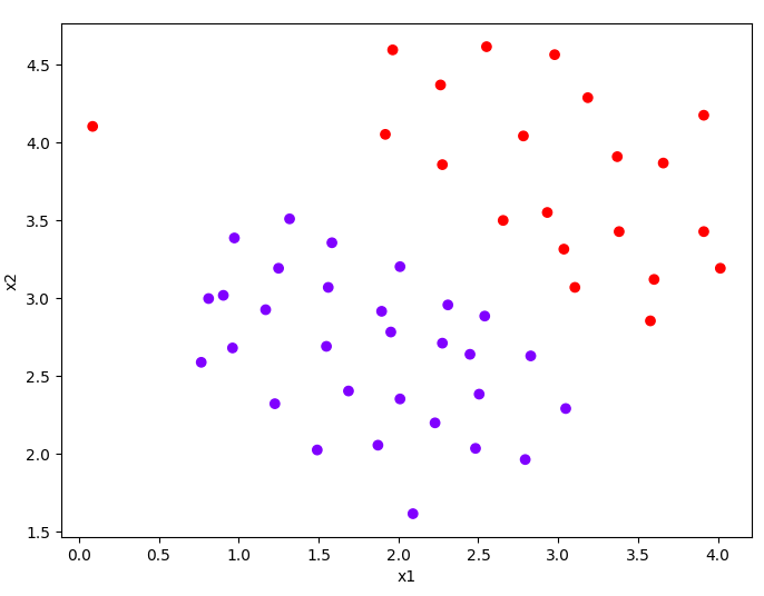

接下来取一段范围,这段范围是根据已有数据的大小进行细微扩大,并且将其分成500段,通过meshgrid获得网格线,最终利用等高线图画出分界线
1.2 Decision Boundary
def plotBoundary(clf, X):
    '''Plot Decision Boundary'''
    x_min, x_max = X[:, 0].min() * 1.2, X[:, 0].max() * 1.1
    y_min, y_max = X[:, 1].min() * 1.1, X[:, 1].max() * 1.1

    xx, yy = np.meshgrid(np.linspace(x_min, x_max, 500), np.linspace(y_min, y_max, 500))
    Z = clf.predict(np.c_[xx.ravel(), yy.ravel()])

    Z = Z.reshape(xx.shape)
    plt.contour(xx, yy, Z)

    pass
通过调用sklearn中支持向量机的代码,来进行模型的拟合
models = [svm.SVC(C, kernel='linear') for C in [1, 100]]

clfs = [model.fit(X, y.ravel()) for model in models]
score = [model.score(X, y) for model in models]
def plot():
    title = ['SVM Decision Boundary with C = {}(Example Dataset 1)'.format(C) for C in [1, 100]]
    for model, title in zip(clfs, title):

        plt.figure(figsize=(8, 5))
        plotData(X, y)
        plotBoundary(model, X)
        plt.title(title)
        pass
    pass
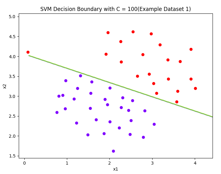
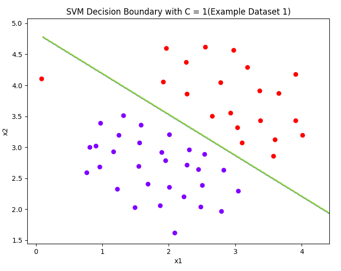
A large C parameter tells the SVM to try to classify all the examples correctly.
C plays a rolesimilar to λ, where λ is the regularization parameter that we were using previously for logistic regression.
可以理解对误差的惩罚,惩罚大,则曲线分类精准。
1.2 SVM with Gaussian Kernels
当用SVM作非线性分类时,我们一般使用Gaussian Kernels。
K gaussian ( x ( i ) , x ( j ) ) = exp ( − ∥ x ( i ) − x ( j ) ∥ 2 2 σ 2 ) = exp ( − ∑ k = 1 ( x k ( i ) − x k ( j ) ) 2 2 σ 2 ) K_{\text {gaussian }}\left(x^{(i)}, x^{(j)}\right)=\exp \left(-\frac{\left\|x^{(i)}-x^{(j)}\right\|^{2}}{2 \sigma^{2}}\right)=\exp \left(-\frac{\sum_{k=1}\left(x_{k}^{(i)}-x_{k}^{(j)}\right)^{2}}{2 \sigma^{2}}\right)K gaussian (x (i ),x (j ))=exp (−2 σ2 ∥∥x (i )−x (j )∥∥2 )=exp ⎝⎜⎛−2 σ2 ∑k =1 (x k (i )−x k (j ))2 ⎠⎟⎞
本文中使用其自带的即可。
def gaussKernel(x1, x2, sigma):
    return np.exp(-(x1 - x2) ** 2).sum() / (2 * sigma ** 2)

a = gaussKernel(np.array([1, 2, 1]), np.array([0, 4, -1]), 2.)
1.2.1 Gaussian Kernel-Example Dataset2
mat = loadmat('data/ex6data2.mat')
x2 = mat['X']
y2 = mat['y']
plotData(x2, y2)
plt.show()
[外链图片转存失败,源站可能有防盗链机制,建议将图片保存下来直接上传(img-ktLdbJ8u-1622612399587)(C:/Users/DELL/AppData/Roaming/Typora/typora-user-images/image-20210601172524887.png)]
sigma = 0.1
gamma = np.power(sigma, -2)/2
'''
高斯核函数中的gamma越大,相当高斯函数中的σ越小,此时的分布曲线也就会越高越瘦。
高斯核函数中的gamma越小,相当高斯函数中的σ越大,此时的分布曲线也就越矮越胖,smoothly,higher bias, lower variance
'''
clf = svm.SVC(C=1, kernel='rbf', gamma=gamma)
model = clf.fit(x2, y2.flatten())
1.2.2 Gaussian Kernel-Example Dataset3
'''
Example Dataset3
'''
mat3 = loadmat('data/ex6data3.mat')
x3, y3 = mat3['X'], mat3['y']
Xval, yval = mat3['Xval'], mat3['yval']
plotData(x3, y3)
Cvalues = (0.01, 0.03, 0.1, 0.3, 1., 3., 10., 30.)
sigmavalues = Cvalues
best_pair, best_score = (0, 0), 0
for C in Cvalues:
for sigma in sigmavalues:
gamma = np.power(sigma, -2.) / 2
model = svm.SVC(C=C, kernel='rbf', gamma=gamma)
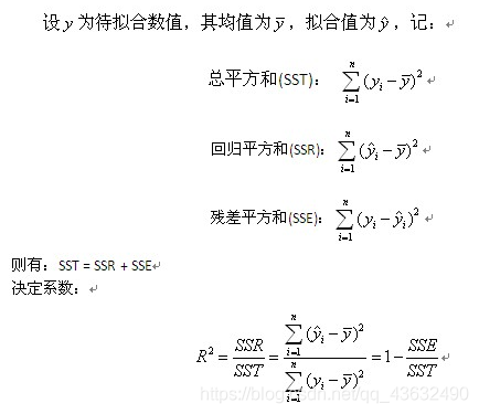
model.fit(x3, y3.flatten())
this_score = model.score(Xval, yval)
'''
model.score函数的返回值是决定系数,也称R2。
可以测度回归直线对样本数据的拟合程度,决定系数的取值在0到1之间,
决定系数越高,模型的拟合效果越好,即模型解释因变量的能力越强。
'''
if this_score > best_score:
best_score = this_score
best_pair = (C, sigma)
pass
pass
print('最优(C, sigma)权值:', best_pair, '决定系数:', best_score)
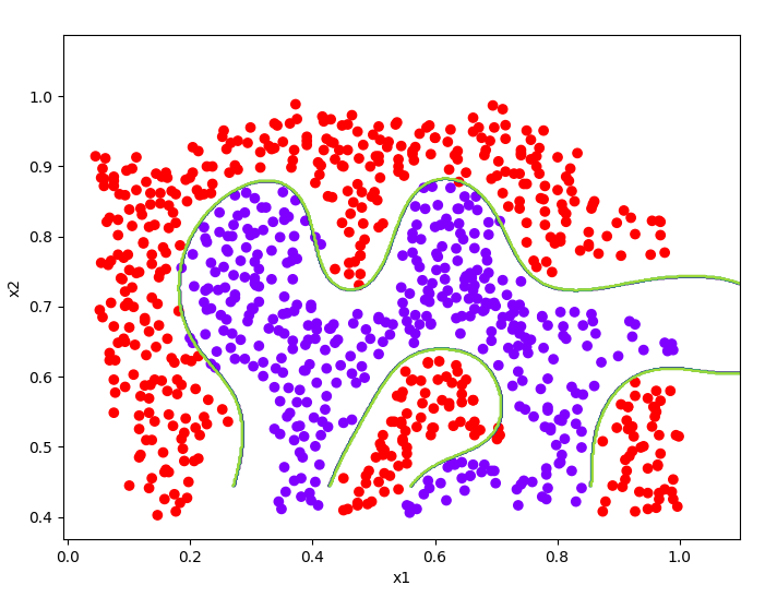
model = svm.SVC(1, kernel='rbf', gamma=np.power(0.1, -2.) / 2)
model.fit(x3, y3.flatten())
plotData(x3, y3)
plotBoundary(model, x3)
[外链图片转存失败,源站可能有防盗链机制,建议将图片保存下来直接上传(img-zODc0dOu-1622612399590)(C:/Users/DELL/AppData/Roaming/Typora/typora-user-images/image-20210601224239696.png)]
SVM中的score的作用:
2 Spam Classfication
邮件分类这一块就偷一下懒拉,给大家看看代码
import numpy as np
import matplotlib.pyplot as plt
from scipy.io import loadmat
from sklearn import svm
import pandas as pd
import re
from stemming.porter2 import stem
import nltk, nltk.stem.porter
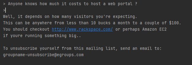
with open('data/emailSample1.txt', 'r') as f:
email = f.read()
pass
print(email)
def processEmail(email):
'''除了Word Stemming, Removal of non-words之外所有的操作'''
email = email.lower()
email = re.sub(']>', '', email)
email = re.sub('(http|https)://[^\s]*', 'httpaddr', email)
email = re.sub('[^\s]+@[^\s]+', 'emailaddr', email)
email = re.sub('[\$]+', 'dollar', email)
email = re.sub('[\d]+', 'number', email)
return email
def email2TokenList(email):
"""预处理数据,返回一个干净的单词列表"""
stemmer = nltk.stem.porter.PorterStemmer()
email = processEmail(email)
tokens = re.split('[ \@\$\/\#\.\-\:\&\*\+\=\[\]\?\!\(\)\{\}\,\'\"\>\_\, email)
tokenlist = []
for token in tokens:
token = re.sub('[^a-zA-Z0-9]', '', token)
stemmed = stemmer.stem(token)
if not len(token):
continue
tokenlist.append(stemmed)
return tokenlist
def email2VocanIndices(email, vocab):
'''提取存在单词的索引'''
token = email2TokenList(email)
index = [i for i in range(len(vocab)) if vocab[i] in token]
return index
def email2FeatureVector(email):
'''
将email转化为词向量,n是vocab的长度。存在单词的相应位置的值置为1,其余为0
:param email:
:return:
'''
df = pd.read_table('data/vocab.txt', names=['words'])
vocab = np.array(df)
vector = np.zeros(len(vocab))
vocab_indices = email2VocanIndices(email, vocab)
for i in vocab_indices:
vector[i] = 1
pass
return vector
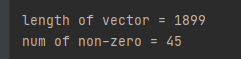
vector = email2FeatureVector(email)
print('length of vector = {}\nnum of non-zero = {}'.format(len(vector), int(vector.sum())))
mat1 = loadmat('data/spamTrain.mat')
X, y = mat1['X'], mat1['y']
mat2 = loadmat('data/spamTest.mat')
Xtest, ytest = mat2['Xtest'], mat2['ytest']
clf = svm.SVC(C=0.1, kernel='linear')
clf.fit(X, y)
predTrain = clf.score(X, y)
predTest = clf.score(Xtest, ytest)
print(predTrain, predTest)
附完整代码:
import numpy as np
import pandas as pd
import matplotlib.pyplot as plt
import seaborn as sb
from scipy.io import loadmat
from sklearn import svm

'''
1.Prepare datasets
'''
mat = loadmat('data/ex6data1.mat')
print(mat.keys())

X = mat['X']
y = mat['y']
'''大多数SVM的库会自动帮你添加额外的特征x0,所以无需手动添加。'''

def plotData(X, y):
    plt.figure(figsize=(8, 6))
    plt.scatter(X[:, 0], X[:, 1], c=y.flatten(), cmap='rainbow')

    plt.xlabel('x1')
    plt.ylabel('x2')

    pass

def plotBoundary(clf, X):
    '''Plot Decision Boundary'''
    x_min, x_max = X[:, 0].min() * 1.2, X[:, 0].max() * 1.1
    y_min, y_max = X[:, 1].min() * 1.1, X[:, 1].max() * 1.1

    xx, yy = np.meshgrid(np.linspace(x_min, x_max, 500), np.linspace(y_min, y_max, 500))
    Z = clf.predict(np.c_[xx.ravel(), yy.ravel()])

    Z = Z.reshape(xx.shape)
    plt.contour(xx, yy, Z)

    pass

models = [svm.SVC(C, kernel='linear') for C in [1, 100]]

clfs = [model.fit(X, y.ravel()) for model in models]
score = [model.score(X, y) for model in models]

def plot():
    title = ['SVM Decision Boundary with C = {}(Example Dataset 1)'.format(C) for C in [1, 100]]
    for model, title in zip(clfs, title):

        plt.figure(figsize=(8, 5))
        plotData(X, y)
        plotBoundary(model, X)
        plt.title(title)
        pass
    pass

'''
2.SVM with Gaussian Kernels
'''

def gaussKernel(x1, x2, sigma):
    return np.exp(-(x1 - x2) ** 2).sum() / (2 * sigma ** 2)

a = gaussKernel(np.array([1, 2, 1]), np.array([0, 4, -1]), 2.)

'''
Example Dataset 2
'''

mat = loadmat('data/ex6data2.mat')
x2 = mat['X']
y2 = mat['y']
plotData(x2, y2)
plt.show()

sigma = 0.1
gamma = np.power(sigma, -2)/2
'''
高斯核函数中的gamma越大,相当高斯函数中的σ越小,此时的分布曲线也就会越高越瘦。
高斯核函数中的gamma越小,相当高斯函数中的σ越大,此时的分布曲线也就越矮越胖,smoothly,higher bias, lower variance
'''
clf = svm.SVC(C=1, kernel='rbf', gamma=gamma)
model = clf.fit(x2, y2.flatten())

'''
Example Dataset3
'''
mat3 = loadmat('data/ex6data3.mat')
x3, y3 = mat3['X'], mat3['y']
Xval, yval = mat3['Xval'], mat3['yval']
plotData(x3, y3)

Cvalues = (0.01, 0.03, 0.1, 0.3, 1., 3., 10., 30.)
sigmavalues = Cvalues
best_pair, best_score = (0, 0), 0

for C in Cvalues:
    for sigma in sigmavalues:
        gamma = np.power(sigma, -2.) / 2
        model = svm.SVC(C=C, kernel='rbf', gamma=gamma)
        model.fit(x3, y3.flatten())
        this_score = model.score(Xval, yval)
        '''
         model.score函数的返回值是决定系数,也称R2。
         可以测度回归直线对样本数据的拟合程度,决定系数的取值在0到1之间,
         决定系数越高,模型的拟合效果越好,即模型解释因变量的能力越强。
         '''

        if this_score > best_score:
            best_score = this_score
            best_pair = (C, sigma)
        pass
    pass
print('最优(C, sigma)权值:', best_pair, '决定系数:', best_score)

model = svm.SVC(1, kernel='rbf', gamma=np.power(0.1, -2.) / 2)

model.fit(x3, y3.flatten())
plotData(x3, y3)
plotBoundary(model, x3)
参考链接:https://blog.csdn.net/Cowry5/article/details/80465922
Original: https://blog.csdn.net/weixin_48577398/article/details/117465475
Author: TCQD
Title: 吴恩达机器学习python实现(6):SVM支持向量机(文末附完整代码)
原创文章受到原创版权保护。转载请注明出处:https://www.johngo689.com/672682/
转载文章受原作者版权保护。转载请注明原作者出处!