Convolutional Neural Networks for Sentence Classification(卷积神经网络句子分类）

目录

摘要

原文

翻译

单词解释

技术解读

引言

原文

翻译

单词解释

技术解读

原文

翻译

单词解释

技术解读

原文

翻译

单词解释

技术解读

原文

翻译

单词解释

技术解读、

Model

原文

单词解释

技术解读

Regularization

原文

单词解释

技术解读

数据集和实验

超参数和模型训练

翻译

涉及技术

dropout技术

l2范数

网格搜索

使用场景

随机梯度下降

梯度下降算法

随机梯度下降算法

预训练词向量

技术解读

预训练词向量

模型变体

本文使用基准模型线索

结论和结果

多通道和单通道

静态和非静态表示

Futher Observation

总结

写作思路

本文写作思路

写作思路

读后心得

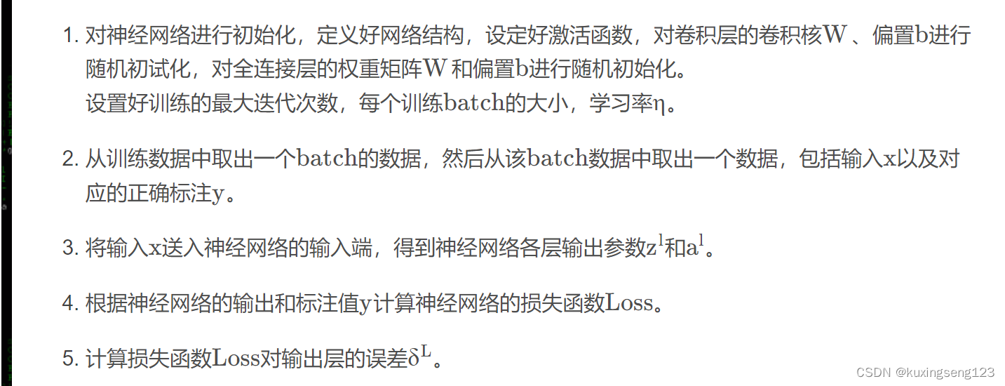
摘要

• *原文

We report on a series of experiments with convolutional neural networks (CNN) trained on top of pre-trained word vectors for sentence-level classification tasks. We show that a simple CNN with little hyperparameter tuning and static vectors achieves excellent results on multiple benchmarks. Learning task-specific vectors through fine-tuning offers further gains in performance. We additionally propose a simple modification to the architecture to allow for the use of both task-specific and static vectors. The CNN models discussed herein improve upon the state of the art on 4 out of 7 tasks, which include sentiment analysis and question classification.

• *翻译

我们报告了一系列在预训练词向量之上训练的卷积神经网络（CNN）实验，用于句子级分类任务。我们表明，几乎没有 超参数调整和静态向量的简单CNN在多个基准上均能获得出色的结果。

通过 微调学习特定任务的向量可进一步提高性能，另外建议对体系结构进行简单的修改，以允许使用 特定任务的向量和静态向量，本文讨论的CNN模型在7个任务中的 4个改进了现有技术，其中包括 情感分析和问题分类。

• *单词解释

a series of 一系列、pre-trained word vectors预训练词向量、

sentence-level classification tasks.句子级分类任务、

hyperparameter tuning 超参数调整

static vectors静态向量。multiple benchmarks多个基准。fine-tuning 微调

the architecture体系、sentiment analysis 情感分析 question classification.问题分类

• *技术解读

超参数：超参数是在 建立模型时用来控制算法行为的参数。这些参数不能从正常的训练过程中学习。他们需要 在训练模型之前被分配。

超参数调整的方法： 网格搜索、随机搜索、贝叶斯调参、手动调参。

预训练词向量方式： Word2Vec、 GLOVE、FastText、n-gram。

sequence-level task（句子级别任务）：

如 情感分类等各种句子分类问题; 推断 两个句子的是否是同义等.（判断两个句子是相近、矛盾、中立）

即给出 一对(a pair of)句子, 判断两个句子是 entailment (相近), contradiction (矛盾)还是 neutral (中立)的. 由于也是分类问题, 也被称为 sentence pair classification tasks.

会自己 找对应任务的相关经典数据集。

静态向量的简单CNN

将一个词在整个语料库中的共现上下文信息聚合至该词的向量表示中，也就是说，对于任意一个词，其向量表示是恒定的， 不随其上下文的变化而变化。（缺陷无法表达多意性）

基准模型：

baseline一词应该指的 是对照组，基准线，就是你这个实验有提升，那么你的提升是对比于什么的提升， 被对比的就是baseline。

引言

• *原文

Deep learning models have achieved remarkable results in computer vision (Krizhevsky et al., 2012) and speech recognition (Graves et al., 2013) in recent years. Within natural language processing, much of the work with deep learning methods has involved learning word vector representations through neural language models (Bengio et al., 2003; Yih et al., 2011; Mikolov et al., 2013) and performing composition over the learned word vectors for classification (Collobert et al., 2011). Word vectors, wherein words are projected from a sparse, 1-of-V encoding (here V is the vocabulary size) onto a lower dimensional vector space via a hidden layer, are essentially feature extractors that encode semantic features of words in their dimensions. In such dense representations, semantically close words are likewise close—in euclidean or cosine distance—in the lower dimensional vector space.

• *翻译

近年来，深度学习模型在计算机视觉（Krizhevsky et al., 2012）和语音识别（Graves et al., 2013）中取得了显著的效果，在自然语言处理中，深度学习方法的许多工作都涉及通过神经语言模型（ Bengio et al., 2003； Yih et al., 2011； Mikolov et al., 2013）来学习词向量表示。

并在学习的词向量进行分类（ Collobert et al., 2011）。词向量本质是特征提取，其将词从稀疏的V编码1（这里V是词汇量）通过 隐藏层投影到较低维度的向量空间上，该特征提取对词在其维度上的语义特征进行编码，在这种密集表示中，语义上相近的词在较低维向量空间中也很相近，（ 如欧几里得或余弦距离）。

• *单词解释

Deep learning models 深度学习模型、remarkable result显著的效果、

computer vision 计算机视觉、speech recognition 语音识别、

Within natural language processing 在自然语言处理中。

much of the work 许多工作、word vector representations词向量表示。

neural language models 神经语言模型、

the learned word vectors for classification 在学习的词向量上进行分类。

a sparse, 1-of-V encoding 稀疏的V编码1

a lower dimensional vector space 较低维度的空间向量。

via a hidden layer 通过隐藏层。 essentially feature extractors 本质是特征提取。

semantic features of words 词的语义特征。

dense representations 密集表示、semantically close words 语义上相近的词。

euclidean or cosine distance 欧几里德距离和余弦相似度距离。

• *技术解读

特征提取：词袋模型、TF-IDF文本、特征提取 、word2vector、GloVe、等

稀疏的词向量编码：

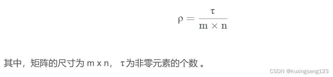
稀疏矩阵的存储

首先何谓 稀疏矩阵，就是在矩阵中有 众多的零元素。稀疏矩阵可以 用稀疏度来进行定量判定。稀疏度的计算公式如下：

稀疏矩阵存储应该满足以下条件：

1. 不存储 0 元素
2. 能够快速恢复到矩阵形态
3. 存储非零元素的数值和位置。

共有三种存储方式： 散居存储、按列/行存储、三角存储

词的语义特征

语义信息：常说的 上下文信息，也就是指一个单词与其周围单词之间的关联。

语义相似度

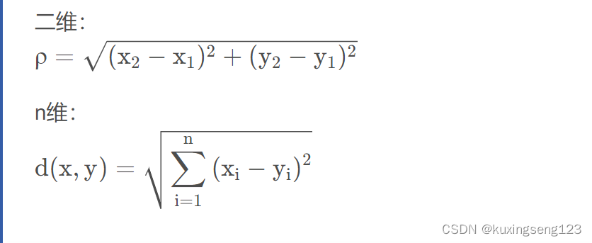
• 欧几里得距离

衡量多维空间中各个点之间得绝对距离，当 数据很稠密并且连续时，这是一种很好得计算方法。

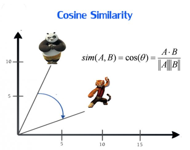
• 余弦相似度 *Cosine Similarity

余弦相似度用 向量空间中两个向量夹角的余弦值作为衡量两 个个体间差异的大小。相比距离度量，余弦相似度更加 注重两个向量在方向上的差异，而非距离或长度上。

一个向量空间中 两个向量夹角间的余弦值作为衡量两个个体之间差异的大小， 余弦值接近1，夹角趋于0，表明两个向量越相似，余弦值接近于0，夹角趋于90度，表明两个向量越不相似。

• 曼哈顿距离 Manhattan Distance
• 明可夫斯基距离（Minkowski distance）
• Jaccard 相似系数（Jaccard Coefficient）
• *斯皮尔曼（等级）相关系数（SRC :Spearman Rank Correlation）

原文

Convolutional neural networks (CNN) utilize layers with convolving filters that are applied to local features (LeCun et al., 1998). Originally invented for computer vision, CNN models have subsequently been shown to be effective for NLP and have achieved excellent results in semantic parsing (Yih et al., 2014), search query retrieval (Shen et al., 2014), sentence modeling (Kalchbrenner et al., 2014), and other traditional NLP tasks (Collobert et al., 2011).

翻译

卷积神经网络（CNN）利用带有卷积滤波器的图层应用于局部特征（LeCun et al., 1998）。 CNN模型最初是为计算机视觉而发明的，后来被证明对NLP有效，并且在语义解析（Yih et al., 2014）、搜索查询检索（Shen et al., 2014）、句子建模（Kalchbrenneret et al., 2014）和其他传统的NLP任务（Collobert et al., 2011）方面取得了优异的结果。
单词解释

local features 局部特征、 layers with convolving filters 带有卷积滤波器的图层。

semantic parsing 语义解析、search query retrieval 搜索查询检索、sentence modeling句子建模
技术解读

传统NLP任务：句子建模、语义解析、搜索查询检索。

CNN技术

主要结构

1. 输入层(Input layer)：输入数据；
2. 卷积层(Convolution layer，CONV)：使用 卷积核进行特征提取和特征映射；
3. 激活层： 非线性映射（ReLU)
4. 池化层(Pooling layer，POOL)：进行下采样降维；
5. 光栅化(Rasterization)：展开像素，与全连接层全连接，某些情况下这一层可以省去；
6. 全连接层(Affine layer / Fully Connected layer，FC)： 在尾部进行拟合，减少特征信息的损失；
7. 激活层：非线性映射（ReLU)
8. 输出层(Output layer)： 输出结果。

其中、卷积层、池化层和激活层可以叠加重复使用，这是CNN的核心结构。

在经过 数次卷积和池化之后，最后会先将 多维的数据进行”扁平化”，也就是把(height,width,channel)的 数据压缩成长度为height × width × channel的一维数组，然后再与FC层连接，这之后就跟 普通的神经网络无异了

卷积层（Convlotuion layer)

卷积层 由一组滤波器组成，滤波器为 三维结构，其深度由输入数据的深度决定，一个滤波器可以看作由 多个卷积核堆叠形成。这 些滤波器在输入数据上滑动做卷积运算，从输入数据中提取特征。在训练时，滤波器上 的权重使用随机值进行初始化，并根据训练集进行学习，逐步优化。

（ 其实就是利用数学公式提取特征类）

1. 卷积运算

卷积核

卷积运算是指以 一定间隔滑动卷积核的窗口，将 各个位置上卷积核的元素和输入的对应元素相乘，然后再 求和（有时将这个计算称为乘积累加运算），将这个 结果保存到输出的对应位置。卷积运算如下所示：

对于一张图像，卷积核从 图像最始端，从左往右、从上往下，以 一个像素或指定个像素的间距依次滑过图像的每一个区域。

​

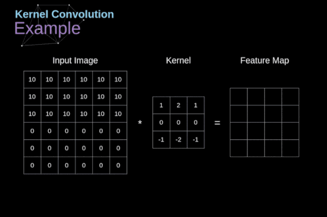
可以把 卷积核理解为权重。每一个 卷积核都可以当做一个”特征提取算子”，把 一个算子在原图上不断滑动，得出的 滤波结果就被叫做”特征图”（Feature Map），这些算子被称为”卷积核”(Convolution Kernel)。我们不必人工设计这些算子，而是 使用随机初始化，来得到很多卷积核，然后通过 反向传播优化这些卷积核，以期望得到更好的识别结果。

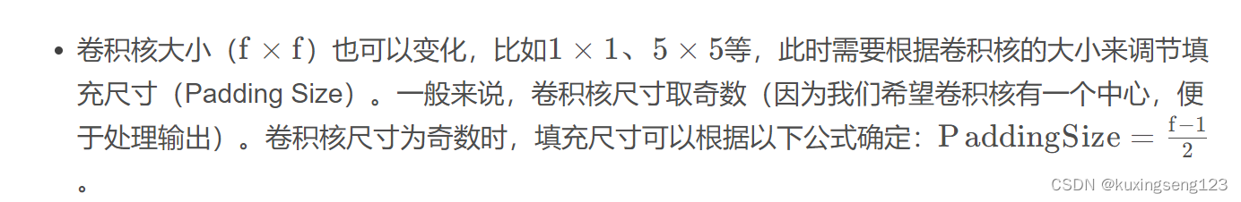
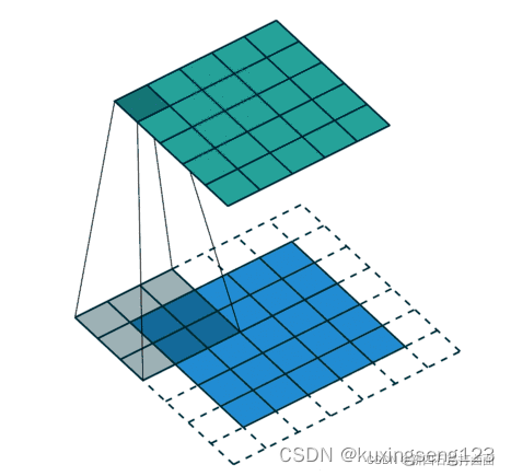
填充/填白（Padding)

在进行 卷积层的处理之前，有时 要向输入数据的周围填入固定的数据（比如0等），使用填充的目的是调 整输出的尺寸，使输出维度和输入维度一致； (输入维度和输出维度一致）

如果 不调整尺寸，经过很多层卷积之后，输出尺寸会变的很小。所以，为 了减少卷积操作导致的，边缘信息丢失，我们就需要进行填充（Padding）。（ 卷积操作导致的边缘信息损失）

步幅与步长（Stride)

• 即 卷积核每次滑动几个像素。前面我们默认 卷积核每次滑动一个像素，其实也可以每次滑动2个像素。其中 ，每次滑动的像素数称为”步长”，步长为2的卷积核计算过程如下；

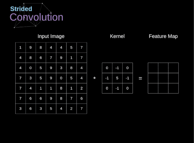
若希望 输出尺寸比输入尺寸小很多，可以采取 增大步幅的措施。但是 不能频繁使用步长为2，因为如果输出尺寸变得过小的话，即 使卷积核参数优化的再好，也会 必可避免地丢失大量信息；

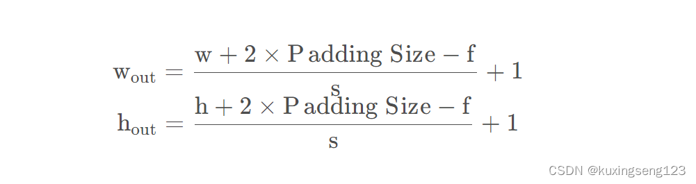
如果用 f 表示卷积核大小，s 表示步长，w 表示图片宽度， h 表示图片高度，那么输出尺寸可以表示为：

滤波器（Fitter)

卷积核（算子） 是二维的权重矩阵；而 滤波器（Filter）是多个卷积核堆叠而成的三维矩阵。

在只有一个通道（二维）的情况下，”卷积核”就相当于”filter”， 这两个概念是可以互换的

上面的卷积过程， 没有考虑彩色图片有RGB三维通道（Channel），如果考虑RGB通道，那么每个通道 都需要一个卷积核，只不过计算的时候 ，卷积核的每个通道在对应通道滑动， 三个通道的计算结果相加得到输出。即：每个滤波器有且只有一个输出通道。

当 滤波器中的各个卷积核在输入数据上滑动时，它们会 输出不同的处理结果，其中一些卷积核的权重可能更高，而 它相应通道的数据也会被更加重视，滤波器会更关注这个通道的特征差异。(滤波器更加关注这个通道的特征差异）

偏置

• 最后，偏置项和滤波器 一起作用产生最终的输出通道。

多个filter也是一样的工作原理：如果存在多个filter，这时 我们可以把这些最终的单通道输出组合成一个总输出，它的 通道数就等于filter数。这个总输出经过 非线性处理后，继续被作为 输入馈送进下一个卷积层，然后重复上述过程。

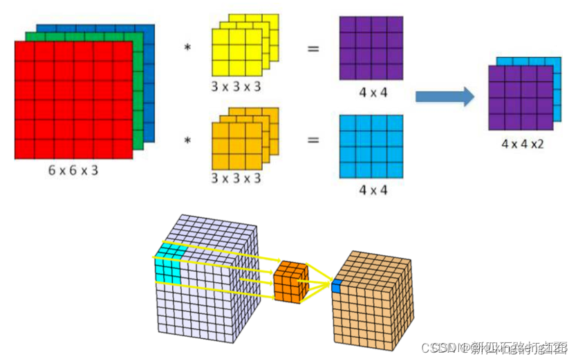
因此，这部分一 共4个超参数： 滤波器数量K ，滤波器大小F ，步长S ，零填充大小P。

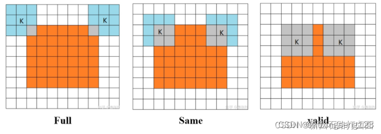
卷积的三种模式

三种卷积模式是对卷积核移动范围的不同限制。

• Full Mode： 从卷积核和图像刚相交时开始做卷积，白色部分填0。
• Same Mode：当 卷积核中心(K)与图像的边角重合时，开始做卷积运算， 白色部分填0。可见其运动范围比Full模式小了一圈。

注意 ：这里的same还有一个意思，卷积之后 输出的feature map尺寸保持不变(相对于输入图片)。当然，same模式 不代表完全输入输出尺寸一样，也跟 卷积核的步长有关系。same模式也是最常见的模式，因为这种模式可以 在前向传播的过程中让特征图的大小保持不变，调参师 不需要精准计算其尺寸变化(因为尺寸根本就没变化)。

• Valid Mode：当 卷积核全部在图像里面时，进行卷积运算，可见其移动范围较Same更小了。

卷积的本质

在具体介绍各种卷积之前，我们有必要再来 回顾一下卷积的真实含义，从数学和图像处理应用的意义上来看一下卷积到底是什么操作。目前大多数深度学习教程 很少对卷积的含义进行细述，大部分只是对 图像的卷积操作进行了阐述。以至于卷积的数学意义和物理意义很多人并不是很清楚，究竟为什么要这样设计，这么设计的原因如何。

追本溯源，我们先回到数学教科书中来看卷积。 在泛函分析中，卷积也叫旋积或者褶积，是一种通过 两个函数x(t)和h(t)生成的数学算子。其计算公式如下：（通过两个函数生成数学算子）

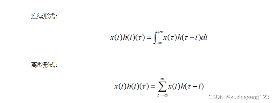
公式写的很清楚了 ，两个函数的卷积就是先将一个函数进行翻转(Reverse)，然后再 做一个平移(Shift)，这便是”卷”的含义。而”积”就是将 平移后的两个函数对应元素相乘求和。所以卷积本质上就是一个Reverse-Shift-Weighted Summation的操作。 （有空搞搞泛函分析）

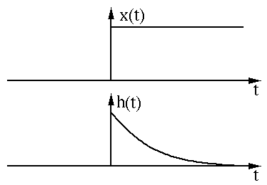
数无形时少直观。我们用 两个函数图像来直观的展示卷积过程和含义。两个函数x(t)和h(t)的图像

如下图所示：

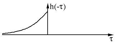
我们先对其中一个 函数h(t)进行翻转(Reverse)操作：

然后进行平移(Shift)：

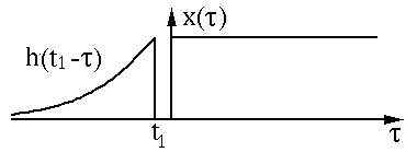
以上过 程是为”卷”。然后是”积”的过程，因为是连续函数，这 里相乘求和为积分形式，图中绿色部分即为相乘求和部分。

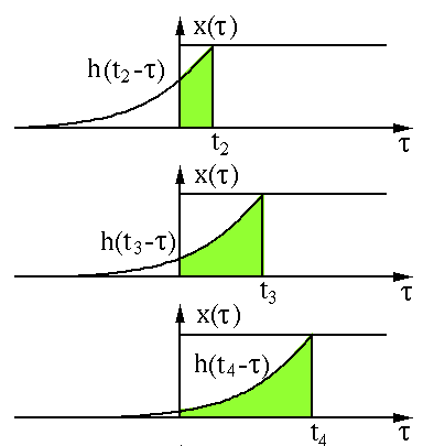
那么为什么要卷积？直接元素相乘不好吗？就 图像的卷积操作而言，笔者认为 卷积能够更好提取区域特征，使用不同大小的卷积算子能够提取图像各个尺度的特征。卷积在 信号处理、图像处理等领域有着广泛的应用。当然，之于深度学习而言，卷积神经网络主要用于图像领域。回顾了卷积的本质之后，我们再来一一梳 理CNN中典型的卷积操作。

具体卷积类型参考链接：

常规卷积：单通道卷积、多通道卷积。

3D卷积、转置卷积、 卷积、深度可分离卷积、空洞卷积。讲解如下

具体卷积类型

池化层（Pooling layer)

池化（Pooling），有的地方也称汇聚， 实际是一个下采样（Down-sample）过程，用来 缩小高、长方向的尺寸，减小模型规模，提高运算速度，同时提高 所提取特征的鲁棒性。简单来说，就是为了 提取一定区域的主要特征，并减少 参数数量，防止模型过拟合。 (减少参数数量，防止模型过拟合）

池化层通常出现在 卷积层之后，二者 相互交替出现，并且 每个卷积层都与一个池化层一一对应。

常用的池化函数有： 平均池化（Average Pooling / Mean Pooling）、最大池化（Max Pooling）、最小池化（Min Pooling）和随机池化（Stochastic Pooling）等，其中3种池化方式展示如下。

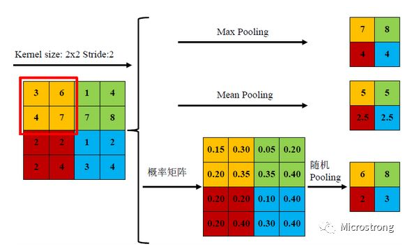
三种池化方式各有优缺点，均值池化是对 所有特征点求平均值，而最大值池化是对 特征点的求最大值。而随机池化则介于两者之间，通过 对像素点按数值大小赋予概率，再按照概率进行亚采样，在平均意义上，与均值采样近似，在局部意义上，则 服从最大值采样的准则。
根据Boureau理论2可以得出结论，在进行 特征提取的过程中，均值池化可以 减少邻域大小受限造成的估计值方差，但更 多保留的是图像背景信息；而 最大值池化能减少卷积层参数误差造成估计均值误差的偏移，能更多的保留纹理信息。随机池化虽然可以保留均值池化的信息，但是随机概率值确是 人为添加的，随机概率的设置对结果影响较大，不可估计。

（ 纹理信息、背景信息）

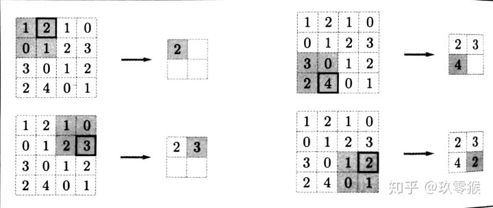
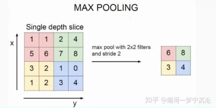
池化操作也有 一个类似卷积核一样东西在特征图上移动，书中叫它 池化窗口3，所以这个池化窗口也有大小，移动的时候有步长， 池化前也有填充操作。因此， 池化操作也有核大小f 、步长s 和填充p 参数，参数意义和卷积相同。Max池化的具体操作如下（池化窗口为2 × 2 ，无填充，步长为2 )：

一般来说， 池化的窗口大小会和步长设定相同的值。

池化层有三个特征：

没有要学习的参数，这和池化层不同。 池化只是从目标区域中取最大值或者平均值，所以没有必要有学习的参数。
通道数不发生改变，即不改变Feature Map的数量。
它是利用 图像局部相关性的原理，对图像进行子抽样，这样对 微小的位置变化具有鲁棒性——输入数据发生微小偏差时，池化仍会 返回相同的结果。

激活层

激活函数：激活函数（Activation Function）运行 时激活神经网络中某一部分神经元，将激活信息向后传入下一层的神经网络。

神经网络中的 每个神经元节点接受上一层神经元的输出值作为本神经元的输入值，并 将输入值传递给下一层，输入层神经元节点会 将输入属性值直接传递给下一层（隐层或输出层）。在多层神经网络中 ，上层节点的输出和下层节点的输入之间具有一个函数关系，这个函数称为激活函数（又称激励函数/传递函数）。

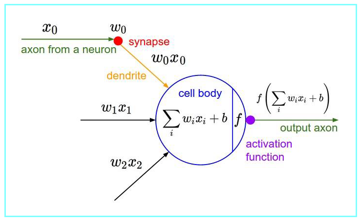
作用： 增加模型的非线性分割能力、提高模型鲁棒性，缓解梯度消失的问题、加速模型收敛等。

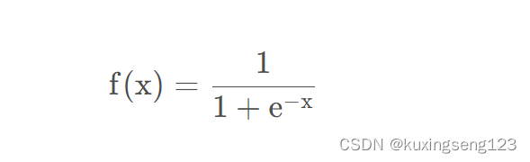
常用激活函数分类：主要分为饱和激活函数、非饱和激活函数。

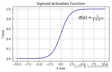
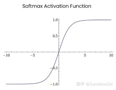
Sigmoid函数

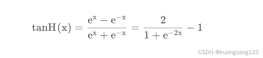
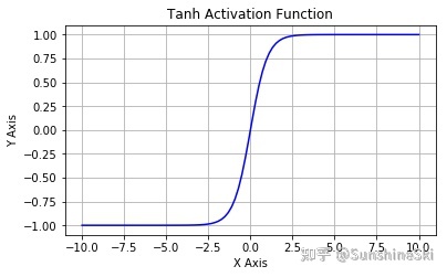
TanH函数

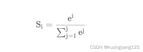
Softmax函数

非饱和激活函数

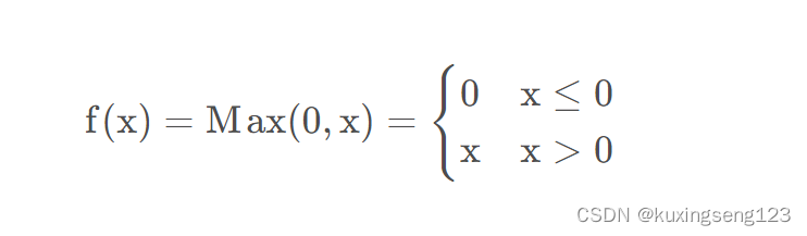
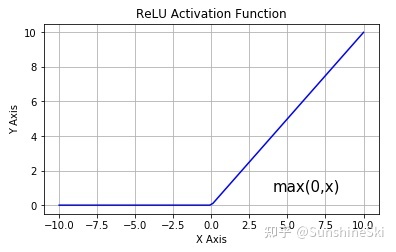
ReLU函数：

激活函数不仅仅以上几种，还有许多不同的激活函数，以上几种是比较常用的，会自己进行总结。活学活用都行啦的样子与打算。激活函数

光栅化

光栅化是把顶点数据转换为片元的过程，具有将图转化为一个个栅格组成的图象的作用，特点是 每个元素对应帧缓冲区中的一像素。

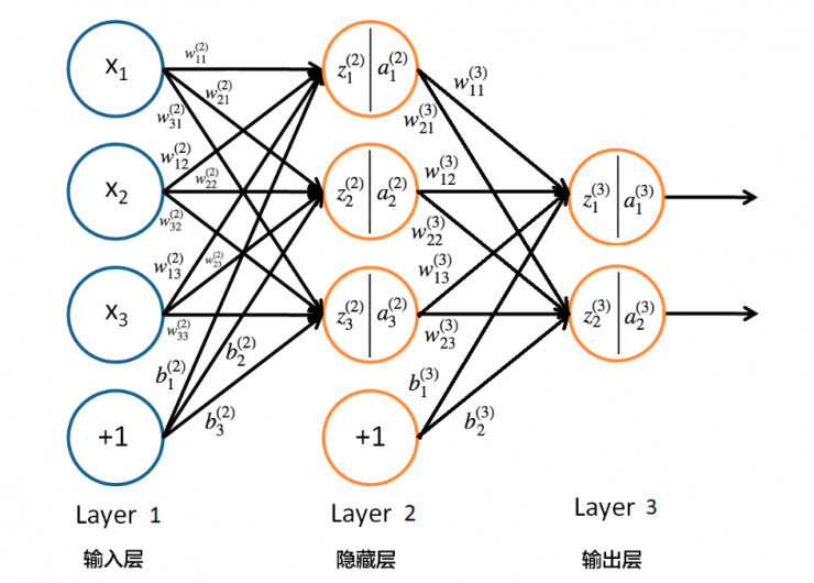
全连接层

可以通过BP网络来理解全连接层， 只不过将 原始数据数据换成以上各层的输出数据。

BP网络

以上总结完成了卷积神经网络的前向传播，有时间将公式全部推导一遍，后续大致梳理其反向传播概述。

反向传播

多层感知机反向传播的数学推导，主要是用数学公式来进行表示的，在全连接神经网络中，它们并不复杂， 即使是纯数学公式也比较好理解，而卷积神经网络反向传播算法相对比较复杂。

卷积神经网络反向传播算法：卷积神经网络反向传播

池化层的反向传播：以最大池化为例

上图中， 池化后的数字6对应于池化前的红色区域，实际上只有 红色区域中最大值数字6对池化后的结果有影响，权重为1，而其它的数字对池化后的结果影响都为0。假设 池化后数字6位置的误差为δ ，反向传播回去时 ，红色区域中最大值对应的位置误差即等于δ ，而其 它3个位置对应的误差为0。

因此，在卷积神经网络最大池化前向传播时， 不仅要记录区域的最大值，同时也要记 录下来区域最大值的位置，方便误差的反向传播。（基于区域最大值位置）

而平均池化就更简单了，由于平均池化时，区域中 每个值对池化后结果贡献的权重都为区域大小的倒数，所以反向传播回来时，在 区域每个位置的误差都为池化后误差除以区域的大小。

（反向传播看权重共享）

卷积的反向传播

虽然 卷积神经网络的卷积运算是一个三维张量的图片和一个四维张量的卷积核进行卷积运算，但最核心的计 算只涉及二维卷积，因此我们先从二维的卷积运算来进行分析：

如上图所示，我们求原图A处的误差，就先分析，它在前向传播中影响了下一层的哪些结点。显然，它只对结点C有一个权重为B的影响， 对卷积结果中的其它结点没有任何影响。因此 A的误差应该等于C点的误差乘上权重B。

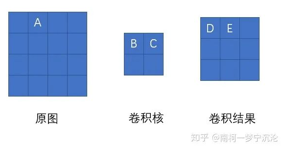
我们现在将 原图A点位置移动一下，则A点以 权重C影响了卷积结果的D点，以权重B影响了卷积结果的E点。那它的误差就等于D点误差乘上C加上E点的误差乘上B。大家可以尝试用相同的方法去分析原图中其它结点的误差，结果会发现， 原图的误差，等于卷积结果的delta误差经过零填充后，与卷积核旋转180度后的卷积。

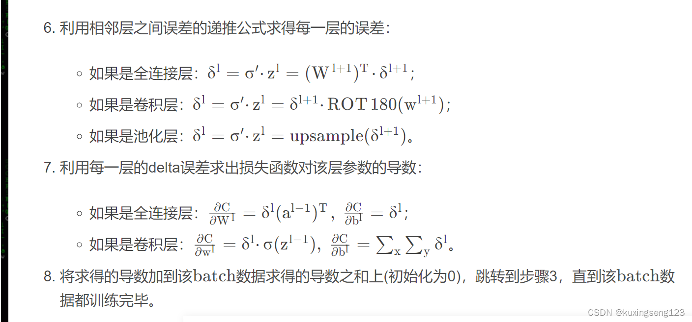
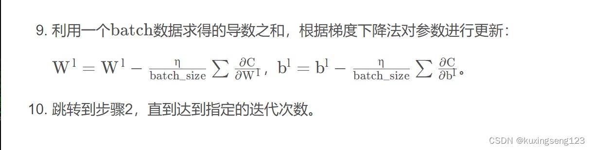
总结卷积神经网络的训练过程

CNN泛化能力提高技巧

增加 神经网络深度；

修改激活函数， 使用较多的是ReLU激活函数；

调整 权重初始化技术，一般来说， 均匀分布初始化效果较好；

调整batch大小（数据集大小）；

扩展 数据集(data augmentation)，可以通过 平移、旋转图像等方式扩展数据集，使学习效果更好；

采取正则化；

采取 Dropout方法避免过拟合。

CNN类型综述

本综述将最近的 CNN 架构创新分为七个不同的类别，分别基于 空间利用、深度、多路径、宽度、特征图利用、通道提升和注意力[^12]。

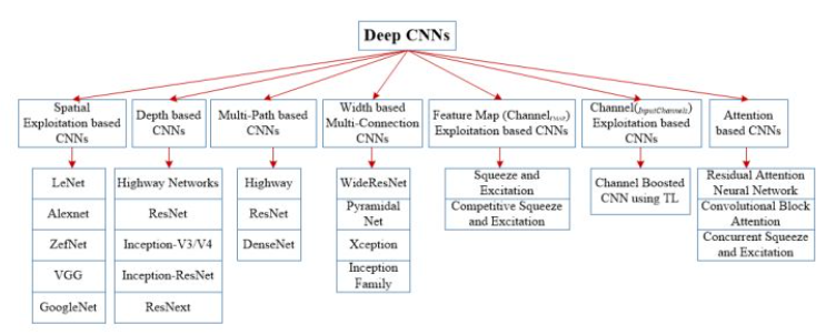
创新视角

参数优化、正则化、结构重组、处理单元的重构和新模块的设计。

引入数据增强、引入注意力、

会自己根据CNN模型来进行文章的编写创新。

tensorflow代码实现CNN

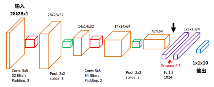
CNN模型的 搭建与搭建全连接层网络的主要步骤是相同的，都是搭建好网络层，定义损失函数和优化之后迭代训练网络。只是网络结构不再只有全连接层，损失函数也 不再使用简单的平方差来定义，并且额外还定义了一种 精确度函数（accuracy）来评判最后模型输出的准确率。因为识别手写数字是有个多分类问题，因此使用的是 softmax分类器，损失函数使用 交叉熵来定义。因为CNN网络的复杂性，CNN模型中也采用了 dropout操作来优化模型。

搭建网络结构：

• 读取mnist数据集数据
• 定义输入输出
• 搭建CNN网络层结构
• 定义损失函数，训练优化最小化损失函数
• *迭代训练模型，评测模型训练结果

import matplotlib.pyplot as plt
import numpy as np
import tensorflow as tf
#下载minist数据集
from tensorflow.examples.tutorials.mnist import input_data
mnist = input_data.read_data_sets('mnist_data',one_hot=True)
#定义输入输出形状
input_x = tf.placeholder(tf.float32,[None,28*28])/255
output_y = tf.placeholder(tf.int32,[None,10])
#输入层，输入数据reshape成四维数据，其中第一维的数据代表了图片数量，因为现在还不清楚图片的数量，因此用-1代替，当传输进数据时python会自动识别出数据的第一维的数值。
input_x_images = tf.reshape(input_x,[-1,28,28,1])
test_x = mnist.test.images[:3000] #读取mnist数据集的测试集图片，读取3000组
test_y = mnist.test.labels[:3000] #读取测试集数据的标签
#第一层结构
#使用2维的卷积层tf.layers.conv2d，使用32个5X5的滤波器，使用relu激活函数
conv1 = tf.layers.conv2d(
inputs=input_x_images,
filters=32,
kernel_size=[5,5],
strides=1,
padding='same',
activation=tf.nn.relu
)
#最大值pooling操作，数据量减半
print(conv1) #输出为[28,28，32]
pool1 = tf.layers.max_pooling2d(
    inputs=conv1,
    pool_size=[2,2],
    strides=2
)
print(pool1) #输出为[14,14,32]
#第二层结构
#使用64个5X5的滤波器
conv2 = tf.layers.conv2d(
inputs=pool1,
filters=64,
kernel_size=[5,5],
strides=1,
padding='same',
activation=tf.nn.relu
)
print(conv2) #输出为[14,14,64]
pool2 = tf.layers.max_pooling2d(
    inputs=conv2,
    pool_size=[2,2],
    strides=2
)
print(pool2) #输出为[7,7,64]
#平坦化操作，将数据变成3136个数据，为全连接层做准备
flat = tf.reshape(pool2,[-1,7*7*64])
#全连接层tf.layers.dense
dense=tf.layers.dense(
    inputs=flat,
    units=1024,
    activation=tf.nn.relu
)
print(dense) #输出为1024个数据
#dropout操作，丢弃率设置为0.5，即一半的神经元丢弃不工作，防止过拟合
dropout = tf.layers.dropout(
    inputs=dense,
    rate=0.5
)
print(dropout) #输出仍为1024个数据，dropout会对输出数据进行scale up
#输出层，就是一个简单的全连接层，没有使用激活函数
outputs = tf.layers.dense(
    inputs=dropout,
    units=10
)
print(outputs) #输出为[10,1]
#使用交叉熵定义损失函数
loss = tf.losses.softmax_cross_entropy(onehot_labels=output_y,logits=outputs)
print(loss)
#训练操作，学习率设置为0.001
train_op = tf.train.GradientDescentOptimizer(0.001).minimize(loss)
#定义精确率，输出预测值与图片标签符合的概率
accuracy_op = tf.metrics.accuracy(
    labels=tf.argmax(output_y,axis=1), #返回张量维度上最大值的索引
    predictions=tf.argmax(outputs,axis=1)
)
print(accuracy_op)
sess=tf.Session()
#初始化所有变量
init=tf.group(tf.global_variables_initializer(),tf.local_variables_initializer())
sess.run(init)
for i in range(20000):
    #取训练的小批次数据，50组数据（图片+标签）
    batch = mnist.train.next_batch(50)
    #训练操作，求训练损失
    train_loss,train_op_=sess.run([loss,train_op],{input_x:batch[0],output_y:batch[1]})
    #每训练迭代100次就输出观察训练的损失函数和测试数据（3000组）的精确度
    if i%100==0:
        #用测试集的数据监测模型训练的效果
        test_accuracy=sess.run(accuracy_op,{input_x:test_x,output_y:test_y})
        print("Step=%d, Train loss=%.4f,Test accuracy=%.2f"%(i,train_loss,test_accuracy[0]))

#测试
test_output=sess.run(outputs,{input_x:test_x[:20]})
inferenced_y=np.argmax(test_output,1)
print(inferenced_y,'Inferenced numbers') #打印输出预测数字
print(np.argmax(test_y[:20],1),'Real numbers') #打印输出标签数字
sess.close()

Step=0, Train loss=0.3977,Test accuracy=0.75
Step=100, Train loss=0.3386,Test accuracy=0.76
Step=200, Train loss=0.2025,Test accuracy=0.76
Step=300, Train loss=0.2278,Test accuracy=0.76
Step=400, Train loss=0.1037,Test accuracy=0.76
Step=500, Train loss=0.3203,Test accuracy=0.77
Step=600, Train loss=0.1972,Test accuracy=0.77
Step=700, Train loss=0.2650,Test accuracy=0.77
Step=800, Train loss=0.3125,Test accuracy=0.77
Step=900, Train loss=0.2740,Test accuracy=0.77
Step=1000, Train loss=0.3872,Test accuracy=0.78
Step=1100, Train loss=0.1174,Test accuracy=0.78
Step=1200, Train loss=0.2942,Test accuracy=0.78
Step=1300, Train loss=0.1785,Test accuracy=0.78
Step=1400, Train loss=0.1765,Test accuracy=0.78
Step=1500, Train loss=0.1228,Test accuracy=0.79
Step=1600, Train loss=0.1618,Test accuracy=0.79
Step=1700, Train loss=0.3901,Test accuracy=0.79
Step=1800, Train loss=0.2776,Test accuracy=0.79
Step=1900, Train loss=0.1562,Test accuracy=0.79
Step=2000, Train loss=0.3695,Test accuracy=0.79
Step=2100, Train loss=0.2548,Test accuracy=0.79
Step=2200, Train loss=0.1935,Test accuracy=0.80
Step=2300, Train loss=0.2357,Test accuracy=0.80
Step=2400, Train loss=0.1429,Test accuracy=0.80
Step=2500, Train loss=0.2501,Test accuracy=0.80
Step=2600, Train loss=0.0757,Test accuracy=0.80
Step=2700, Train loss=0.1751,Test accuracy=0.80
Step=2800, Train loss=0.1364,Test accuracy=0.80
Step=2900, Train loss=0.1119,Test accuracy=0.81
Step=3000, Train loss=0.1932,Test accuracy=0.81
Step=3100, Train loss=0.0863,Test accuracy=0.81
Step=3200, Train loss=0.1375,Test accuracy=0.81
Step=3300, Train loss=0.2874,Test accuracy=0.81
Step=3400, Train loss=0.2263,Test accuracy=0.81
Step=3500, Train loss=0.2988,Test accuracy=0.81
Step=3600, Train loss=0.2046,Test accuracy=0.82
Step=3700, Train loss=0.0886,Test accuracy=0.82
Step=3800, Train loss=0.1063,Test accuracy=0.82
Step=3900, Train loss=0.2221,Test accuracy=0.82
Step=4000, Train loss=0.1758,Test accuracy=0.82
Step=4100, Train loss=0.1478,Test accuracy=0.82
Step=4200, Train loss=0.3418,Test accuracy=0.82
Step=4300, Train loss=0.1630,Test accuracy=0.82
Step=4400, Train loss=0.2907,Test accuracy=0.82
Step=4500, Train loss=0.1294,Test accuracy=0.82
Step=4600, Train loss=0.1838,Test accuracy=0.83
Step=4700, Train loss=0.2521,Test accuracy=0.83
Step=4800, Train loss=0.1400,Test accuracy=0.83
Step=4900, Train loss=0.3340,Test accuracy=0.83

迭代结果都是这样，明天把代码都给其搞一搞，把代码给其研究透彻，全部都将其搞懂都行啦的回事与打算。

原文

In the present work, we train a simple CNN with one layer of convolution on top of word vectors obtained from an unsupervised neural language model. These vectors were trained by Mikolov et al. (2013) on 100 billion words of Google News, and are publicly available.1 We initially keep the word vectors static and learn only the other parameters of the model. Despite little tuning of hyperparameters, this simple model achieves excellent resultson multiple benchmarks, suggesting that the pre-trained vectors are ‘universal’ feature extractors that can be utilized for various classification tasks. Learning task-specific vectors through fine-tuning results in further improvements. We finally describe a simple modification to the architecture to allow for the use of both pre-trained and task-specific vectors by having multiple channels.（多个通道）

翻译

在目前的工作中，我们训练一个简单的CNN,从 无监督神经语言模型得到的词向量的基础上进行一层卷积。这些向量由Mikolov et al.,（2013）训练关于 Google新闻的1000亿个单词，并且已经公开可用。 我们最初使词向量保持静态，仅学习模型的其他参数。 尽管对超参数的调整很少，但这个简单的模型在 多个基准上均能获得出色的结果，这表明预训练的向量是 “通用”特征提取，可用于各种分类任务。通过 微调学习特定任务的向量可以进一步改进。最后，我们描述了对体系结构的简单修改，以允许通过具有多个通道使用预训练向量和特定任务的向量。
单词解释

the present work 目前的工作、
an unsupervised neural language model. 无监督神经语言模型
keep the word vectors static 保持词向量静态。
various classification tasks. 各种分类任务。
task-specific vectors 特定任务的向量。
技术解读

本文没有 什么相关技术，但是有一条重要的写作思路：预训练词向量必须在多个基准模型上看其表现，然后表明其是否可以用于特征提取。

本文说明了经典数据集： Gooogle 新闻1000亿个单词。
原文

Our work is philosophically similar to Razavian et al. (2014) which showed that for image classification, feature extractors obtained from a pretrained deep learning model perform well on a variety of tasks—including tasks that are very different from the original task for which the feature extractors were trained.

翻译

我们的工作在哲学上与Razavian et al. (2014)相似，这表明，对于图像分类，从预训练的深度学习模型中获得的特征提取在各种任务上表现良好，包括与训练特征提取的原始任务截然不同的任务。
单词解释

philosophically 哲学上、 image classification, 图像分类、

the original task 原始任务、
技术解读、

本段没有涉及相关技术，但是要学会慢慢的积累nlp各个领域的相关知识点与技术解读，争取往自己的顶会期刊上靠拢。

Model

原文

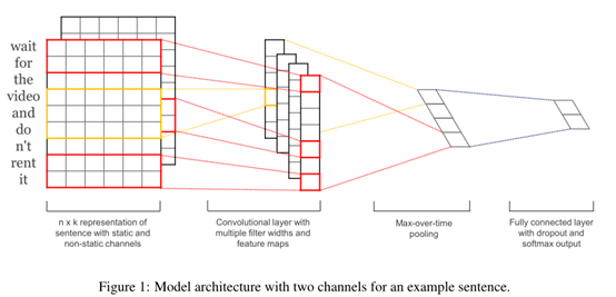
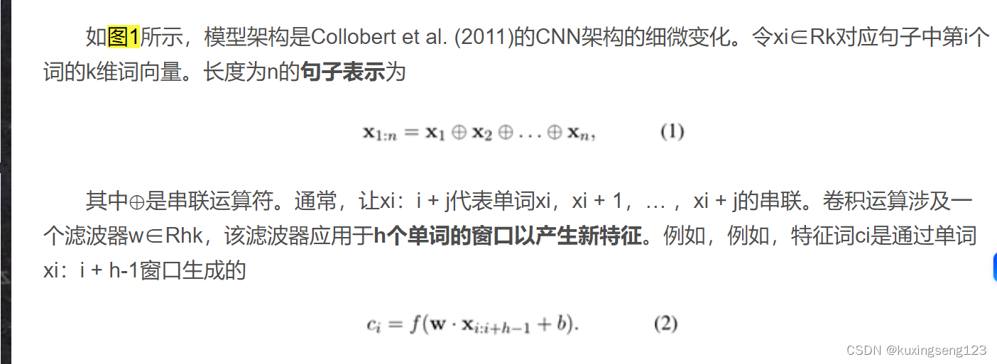
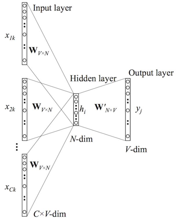
The model architecture, shown in figure 1, is a slight variant of the CNN architecture of Collobert et al. (2011). Let xi ∈ R k be the k-dimensional word vector corresponding to the i-th word in the sentence. A sentence of length n (padded where necessary) is represented as

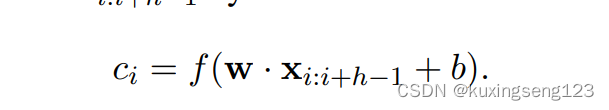
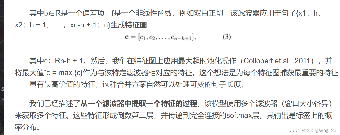
here ⊕ is the concatenation operator. In general, let xi:i+j refer to the concatenation of words xi , xi+1, . . . , xi+j . A convolution operation involves a filter w ∈ R hk, which is applied to a window of h words to produce a new feature. For example, a feature ci is generated from a window of words xi:i+h−1 by：

Here b ∈ R is a bias term and f is a non-linear function such as the hyperbolic tangent. This filter is applied to each possible window of words in the sentence {x1:h, x2:h+1, . . . , xn−h+1:n} to produce a feature map

c = [c1, c2, . . . , cn−h+1],

with c ∈ R n−h+1. We then apply a max-over time pooling operation(Collobert et al., 2011) over the feature map and take the maximum value cˆ = max{c} as the feature corresponding to this particular filter. The idea is to capture the most important feature—one with the highest value—for each feature map. This pooling scheme naturally deals with variable sentence lengths. We have described the process by which one feature is extracted from one filter. The model uses multiple filters (with varying window sizes) to obtain multiple features. These features form the penultimate layer and are passed to a fully connected softmax layer whose output is the probability distribution over labels.

In one of the model variants, we experiment with having two ‘channels’ of word vectors—one

that is kept static throughout training and one that is fine-tuned via backpropagation (section 3.2).2 In t he multichannel architecture, illustrated in figure 1, each filter is applied to both channels and the results are added to calculate ci in equation (2). The model is otherwise equivalent to the single channel architecture.（单通道体系结构）

翻译

在一种模型变体中，我们尝试 使用两个词向量的”通道”，一个在整个训练过程中保持静态，另一个通过反向传播进行微调（第3.2节）。在多通道架构中，如图1所示，每个滤波器都应用于两个通道，并且将结果相加以通过公式（2）计算ci。该模型在其他方面等效于单通道体系结构。

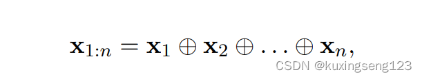
一句话中， n个词，每个词向量长度为k，所有词向量级联，得到n*k的矩阵
卷积操作是 一个窗口长度为h个词的卷积核，对句子做卷积得到新的特征
w为卷积核参数，b为偏置，f为 非线性函数，产生的特征是c
然后对 c使用最大池化，只保留一个 卷积核结果的最大值，即 最重要的特征
通过 多个卷积核得到多个特征，然后进入全连接层（softmax），从而得到每种 分类的概率
实验中尝试了两个通道的词向量，一个保持不变，一个通过反向传播来微调。

单词解释

a slight variant 细微变化、
the k-dimensional word vector k维词向量、
corresponding to the i-th word in the sentence 对应于句子中的第i个词。
the concatenation operator 串联运算符、
the concatenation of words 单词的串联
applied to a window of h words to produce a new feature 滤波器被用于h个单词的窗口以产生新特征。
bias term 偏置项、 non-linear function 非线性函数、
the hyperbolic tangent. 双曲正切、 feature map 特征图、
a max-over time pooling operation 最大超时池化操作
the feature corresponding to this particular filter. 特定滤波器相对应的特征
variable sentence lengths 可变句子长度、 with varying window sizes 窗口大小各异、
the penultimate layer 倒数第二层、
a fully connected softmax layer 全连接softmax层、
the probability distribution over labels. 标签输出是一个概率分布。the model variants 模型变体
技术解读

本段讲解了模型的基本架构， 卷积操作——池化操作——全连接softmax操作。

Regularization

原文

For regularization we employ dropout on the penultimate layer with a constraint on l2-norms of the weight vectors (Hinton et al., 2012). Dropout prevents co-adaptation of hidden units by randomly dropping out—i.e., setting to zero—a proportion p of the hidden units d uring foward backpropagation. That is, given the penultimate layer z = [ˆc1, . . . , cˆm] (note that here we have m filters), i nstead of using

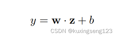
for output unit y in forward propagation, dropout uses

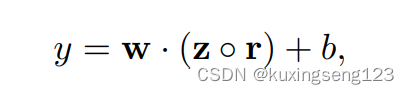
where ◦ is the element-wise multiplication operator and r ∈ R m is a ‘masking’ vector of Bernoulli random variables with probability p of being 1. Gradients are backpropagated only through the unmasked units. At test time, the learned weight vectors are scaled by p such that wˆ = pw, and wˆ is used (without dropout) to score unseen sentences.We additionally constrain l2-norms of the weight vectors by rescaling w to have ||w||2 = s whenever ||w||2 > s after a gradient descent step.

• 在倒数 第二层加入dropout ，并且在词 向量上添加l2范数
• 随机dropout 防止了 隐藏层单元的耦合
• 最大池化后的结果z，与一个 伯努利分布的r对位想乘（为1的概率p），梯度反向传播只经过保留的单元，所以学习 到的权重都乘以了p，乘p后的w用于测试。
• 同时限制l2范数为s

单词解释

co-adaptation of hidden units 隐藏层单元的耦合
技术解读

dropout技术阻止隐藏层单元的耦合。

数据集和实验

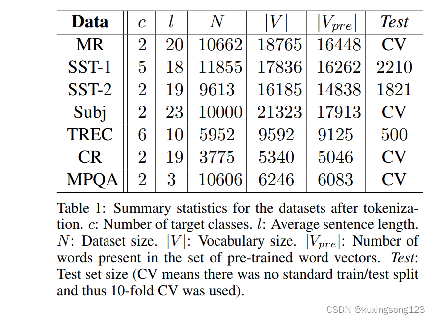
We test our model on various benchmarks. Summary statistics of the datasets are in table 1.

MR: Movie reviews with one sentence per review. Classification involves detecting positive/negative reviews (Pang and Lee, 2005).3
SST-1: Stanford Sentiment Treebank—an extension of MR but with train/dev/test splits provided and fine-grained labels (very positive, positive, neutral, negative, very negative), re-labeled by Socher et al. (2013).4
SST-2: Same as SST-1 but with neutral reviews removed and binary labels.

Subj: Subjectivity dataset where the task is to classify a sentence as being subjective or objective (Pang and Lee, 2004).

TREC: TREC question dataset—task involves classifying a question into 6 question types (whether the question is about person, location, numeric information, etc.) (Li and Roth, 2002).5
CR: Customer reviews of various products (cameras, MP3s etc.). Task is to predict positive/negative reviews (Hu and Liu, 2004).6
MPQA: Opinion polarity detection subtask of the MPQA dataset (Wiebe et al., 2005).7

超参数和模型训练

For all datasets we use: rectified linear units, filter windows (h)of 3, 4, 5 with 100 feature maps each, dropout rate (p) of 0.5, l2 constraint (s) of 3, and mini-batch size of 50. These values were chosen via a grid search on the SST-2 dev set. We do not otherwise perform any dataset specific tuning other than early stopping on dev sets. For datasets without a standard dev set we randomly select 10% of the training data as the dev set. Training is done through stochastic gradient descent over shuffled mini-batches with the Adadelta update rule (Zeiler, 2012).

翻译

1. 使用整流线性单元（ReLU）
2. 卷积核长度分别为3，4，5，每种100个
3. dropout 率为0.5
4. l2范数限制为3
5. 批量大小为50
6. 通过SST-2数据集网格搜索得到这些参数
7. 没有任何针对特殊数据集的微调
8. 对没有验证集的数据从训练集挑选10%
9. 用随机梯度下降训练

涉及技术

dropout技术

这个技 术就是普通的Dropout技术了，Dropout 随机失活神经元，就是我们给出一个概率，让 神经网络层的某个神经元权重为0(失活)

就是每一层， 让某些神经元不起作用，这样就就相当于把网络 进行简化了(左边和右边可以对比），我们有时候之所以会出现过拟合现象，就是因为我们的网络太复杂了，参数太多了，并且我们后面层的网络也可能太过于依赖前层的某个神经元。
加入Dropout之后， 首先 网络会变得简单，减少一些参数，并且由于不知道浅层的哪些神经元会失活，导致后 面的网络不敢放太多的权重在前层的某个神经元，这样就减轻了一个过渡依赖的现象， 对特征少了依赖， 从而有利于缓解过拟合。
创新思维：
Dropout技术的概率p可以用伯努利分布产生。
l2范数

网格搜索

网格搜素是一种 常用的调参手段，是一种 穷举方法。给定一系列超参，然后再所有超参组合中穷举遍历，从 所有组合中选出最优的一组超参数，其实就是 暴力方法在全部解中找最优解。
为什么叫网格搜索，因为假 设有两个超参，每个超参都有一组候选参数。这两组候选参数可以两两组合，把 所有组合列出来就是一个二维的网格（多个超参两两组合可以看作是岗高维空间的网格） ，遍历网格中的所有节点，选出最优解。所以叫网格搜索。

使用场景

网格搜索可以 使用在机器学习算法调参中，而 很少使用在深度神经网络的调参中。因为网络搜索其实并没有什么特别的优化方法， 就是简单的穷举。这种方法不使用网格搜索手动去穷举也是可以实现的 ，只不过网格搜索自动化一些，不需要手工的去一个一个尝试参数。本质就是把所有参数的可能都运行了一遍，对于深度神经网络来说，运行一遍需要很长时间，穷举的去调参，效率太低， 更何况随着超参数数量的增加，超参组合呈几何增长。而对于机器学习的算法来说，运行时间相对较短，甚至对于 朴素贝叶斯这种算法不需要去多次迭代所有样本，训练时间很快，可以使用网格搜索来调参。

随机梯度下降

梯度下降算法

对于神经网络模型来说，如何能 达到高准确率的效果，其关键在于 不断优化目标损失函数，找到近似 最优权重参数，使得 预测估计值不断逼近真实值。
在数学中，我们可以 求得函数y=f(x)的极值点，也就求 它的导数f′(x)=0f的那个点。因此可以通过 解方程f′(x)=0f′(x)=0，求得函数的极值点(x0,y0)(x0,y0)
但是计算机不想人脑一样，可以解方程。但是它可以凭借强大的计算能力，一步一步的把函数的极值点试出来。如下图所示，首先 随机选择一点开始比如x0x0，然后通 过步长不断迭代修改xx后达到

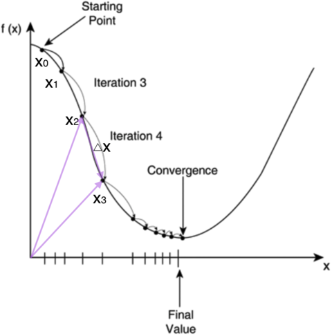
随机梯度下降算法

预训练词向量

Initializing word vectors with those obtained from an unsupervised neural language model is a popular method to improve performance in the absence of a large supervised training set (Collobert et al., 2011; Socher et al., 2011; Iyyer et al., 2014). We use the publicly available word2vec vectorsthat were trained on 100 billion words from Google News. The vectors have dimensionality of 300 and were trained using the continuous bag-of-words architecture (Mikolov et al., 2013). Words not present in the set of pre-trained words are initialized randomly

• 当没有大量有监督训练集时，将词向量初始化为从无监督神经语言模型得到的向量是种广泛的方法
• 用google新闻 的1000亿单词训练得到词向量
• 300维度词向量，用 连续词袋模型训练
• 未出现在 训练集的单词随机初始化*
  技术解读 **

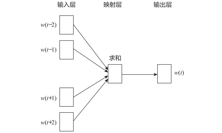
word2vec（连续词袋模型（CBOW)、Skip-gram模型）

根据 上下文预测目标值：对于每一 个单词或词（统称为标识符），使用该标识符周围的标识符来 预测当前标识符生成的概率。假设目标值为”2点钟”，我们可以使用”2点钟”的上文”今天、下午”和”2点钟”的下文”搜索、引擎、组” 来生成或预测目标值。
由 目标值预测上下文：对于每一个标识符，使用 该标识符本身来预测生成其他词汇的概率。如使用”2点钟”来预测其上下文”今天、下午、搜索、引擎、组”中的每个词。
两种预测方法的共同限制条件是 ，对于相同的输入，输出每个标识符的概率之和为1。它们分别对应word2vec的两种模型，即 连续词袋模型（CBOW, The Continuous Bag-of-Words Model）和Skip-Gram模型。根据上下文生成目标值时，使用CBOW模型；根据目标值生成上下文时，采用Skip-Gram模型。
CBOW模型架构

预训练词向量

Initializing word vectorswith those obtained from an unsupervised neural language model is a popular method to improve performance in the absence of a large supervised training set (Collobert et al., 2011; Socher et al., 2011; Iyyer et al., 2014). We use the publicly available w ord2vec vectors that were trained on 100 billion words from Google News. The vectors have dimensionality of 300 and were trained using the continuous bag-of-words architecture (Mikolov et al., 2013). Words not present in the set of pre-trained words are initialized randomly

缺少大量标注数据，通过无监督训练语 料进行词向量的预训练是提升模型表现的常用方法 (Collobert et al.,2011; Socher et al., 2011; Iyyer et al., 2014)，我们使用 公开的预训练词向量，该词向量通过1000亿google新闻单词训练，维度为300，并通过 词袋结构进行训练，未出现在预训练中的 词向量进行随机初始化。

• 当 没有大量有监督训练集时，将词向量初始化为从 无监督神经语言模型得到的向量是种广泛的方法
• 用google新闻的1000亿单词训练得到词向量
• 300维度词向量，用 连续词袋模型训练
• 未出现在 训练集的单词随机初始化

模型变体

CNN-rand: Our baseline model where all words are randomly initialized and then modified during training.

CNN-static: A model with pre-trained vectors from word2vec. All words including the unknown ones that are randomly initialized—are kept static and only the other parameters of the model are learned.

CNN-non-static: Same as above but the pretrained vectors are fine-tuned for each task.

CNN-multichannel: A model with two sets of word vectors. Each set of vectors is treated as a ‘channel’ and each filter is applied to both channels, but gradients are backpropagated only through one of the channels. Hence the model is able to finetune one set of vectors while keeping the other static. Both channels are initialized with word2vec.

本文使用基准模型线索

1. 初始化词向量
2. word2vec预训练词向量
3. 词向量训练中迭代修改。
4. 使用两通道词向量

结论和结果

Results of our models against other methods are listed in table 2. Our baseline model with all randomly initialized words (CNN-rand) does not perform well on its own. While we had expected performance gains through the use of pre-trained vectors, we were surprised at the magnitude of the gains. Even a simple model with static vectors (CNN-static) performs remarkably well, giving competitive results against the more sophisticated deep learning models tha t utilize complex pooling schemes(Kalchbrenner et al., 2014) or require parse trees to be computed beforehand(Socher et al., 2013). These results suggest that the pretrained vectors are good, ‘universal’ feature extractors and can be utilized across datasets. Finetuning the pre-trained vectors for each task gives still further improvements (CNN-non-static).

模型实验结果对比见表2。模型的baseline随机初始化词向量（CNN-rand）并未表现最佳，预期使用预训练词向量可以提升效果，但结果幅度惊人。即使带有静态向量的简单模型（CNN-static）也表现不错，但对比使用复杂池化方案的复杂深度模型或事先计算解析树的应用，这些结果表明进行预训练的词向量是 通用的特征提取器，能在不同数据集中使用，根据具体任务对预训练词向量进行微调又能进一步改进效果。

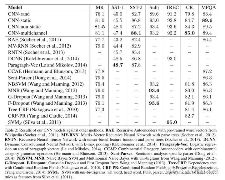
• 随机初始化词向量性能不好
• 基于预训练词向量的改善比较大
• 每个任务中微调词向量性能更好

多通道和单通道

We had initially hoped that the multichannel architecture would prevent overfitting (by ensuring that the learned vectors do not deviate too far from the original values) and thus work better than the single channel model, especially on smaller datasets. The results, however, are mixed, and further work on regularizing the fine-tuning process is warranted. For instance, instead of using an additional channel for the non-static portion, one could maintain a single channel but employ extra dimensions that are allowed to be modified during training.

初始阶段 思考多通道结构能防止过拟合，尤其在 小数据上能比单通道表现更好，但实验结果并非绝对，因此 有必要进一步规范微调过程，例如代替使用 非静态的附加通道，保持单通道，但训 练期间可以进行维度调整。

静态和非静态表示

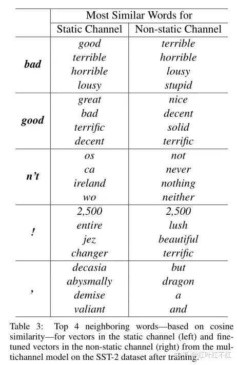
As is the case with t he single channel non-static model, the multichannel model is able to fine-tune the non-static channel to make it more specific to the task-at-hand. For example, good is most similar to bad in word2vec, presumably because they are (almost) syntactically equivalent. But for vectors in the non-static channel that were finetuned on the SST-2 dataset, this is no longer the case (table 3). Similarly, good is arguably closer to nice than it is to great for expressing sentiment, and this is indeed reflected in the learned vectors. For (randomly initialized) tokens not in the set of pre-trained vectors , fine-tuning allows them to learn more meaningful representations: the network learns that exclamation marks are associated with effusive expressions and that commas are conjunctive (table 3).

和单通道非静态模型类似， 多通道能对非静态通道进行微调，使之更适用于具体任务。比如，good和bad在word2vec中非常类似，因为其在句法上是等价的，但在 SST-2数据集上非静态通道进行微调，情况就不是如此（表3），类似在情绪表达上good相对great要跟更接近nice，这 在学习到的向量中也的确得到体现。对于不在预训练范围的随机初始化词向量， 微调能使其学到更有意义的表征，如感叹号与情绪相关，逗号作为连词。

Futher Observation

Kalchbrenner et al. (2014) report much worse results with a CNN that has essentially the same architecture as our single channel model. Forexample, theirMax-TDNN(Time Delay Neural Network) with randomly initialized words obtains 37.4% on the SST-1 dataset, compared to 45.0% for our model. We attribute such discrepancy to our CNN having much more capacity (multiple filter widths and feature maps).

Dropout proved to be such a good regularizer that it was fine to use a larger than necessary network and simply let dropout regularize it. Dropout consistently added 2%–4% relative performance.

When randomly initializing words not in word2vec, we obtained slight improvements by sampling each dimension from U[−a,a] where a was chosen such that the randomly initialized vectors have the same variance as the pre-trained ones. It would be interesting to see if employing more sophisticated methods to mirror the distribution of pre-trained vectors in the initialization process gives further improvements.

We briefly experimented with another set of publicly available word vectors trained by Collobert et al. (2011) on Wikipedia, 8 and found that word2vec gave far superior performance. It is not clear whether this is due to Mikolov et al. (2013)’s architecture or the 100 billion word Google News dataset.

Adadelta (Zeiler, 2012) gave similar results to Adagrad (Duchi et al., 2011) but required fewer epochs.

总结

构建词向量的方式： 基于预训练模型、随机初始化词向量、微调词向量。 两通道词向量
写作思路****

以证明某种观点为主线来设计不同模型，在不同数据上进行性能测试。

1. much worse results with a CNN that has essentially the same architecture as our single channel model
2. Dropout proved to be such a good regularizer
3. gave similar results to Adagrad (Duchi et al., 2011) but required fewer epochs.
4. 这些结果表明进行预训练的词向量是 通用的特征提取器，能在不同数据集中使用，根据具体任务对预训练词向量进行微调又能进一步改进效果。

本文写作思路

使用不同的方式来构建预训练词向量，并测试多个模型，在不同数据集上测试性能，依次来证明预训练的词向量是 通用的特征提取器，能在不同数据集中使用，根据具体任务对预训练词向量进行微调又能进一步改进效果

写作思路****

证明某种观点——自己构建不同的模型在数据集上测试性能。

会自己构建基准模型，并进行不同的优化。

读后心得

会有利用该层的误差求得梯度函数的导数的思维。

会根据某一基准模型和综述开发出自己的模型，并用代码和数据集检测。

针对某一架构进行创新。

会自己总结论文中的创新思路。

训练词向量在多个基准上进行训练，会自己看看效果。

设计模型的时候，会自己找评价指标与多个基准模型，来评价预训练词向量的质量。

会了解词向量组成句子的表示方法

其实论文模型部分就是把你做实验的步骤以及过程都给详细推导出来，重点是指明使用的那种技术是谁提出的。

单词的维度什么的都必须将其搞清楚，相当的重要。

论文思路是从那来的，真心特别俩像了节

为什么使用这一步，为什么使用那一步，相当的重要。

后期，不断研究下代码，把代码给其研究透彻，升级下自己的思路。并不断的复现论文。

争取发现自己的写作点。冲刺顶刊！

Original: https://blog.csdn.net/kuxingseng123/article/details/127274912
Author: big_matster
Title: Convolutional Neural Networks for Sentence Classification(卷积神经网络句子分类）