

文章目录
神经网络架构
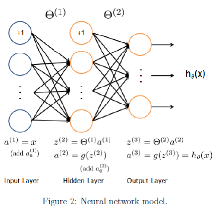

分为三层,输入层、隐藏层与输出层。输入层为400个单元分别对应手写数字图片中的400个像素,隐藏层有25个单元,输出层有10个单元对应10个数字。
输入矩阵X X X为5000×400的矩阵,包含5000张手写数字图片,每张图片有20×20=400个像素。
X = [ − ( x ( 1 ) ) T − − ( x ( 2 ) ) T − ⋮ − ( x ( m ) ) T − ] X=\left[\begin{matrix} -(x^{(1)})^T-\ -(x^{(2)})^T-\ \vdots\ -(x^{(m)})^T-\ \end{matrix}\right]X =⎣⎢⎢⎢⎡−(x (1 ))T −−(x (2 ))T −⋮−(x (m ))T −⎦⎥⎥⎥⎤
对于答案矩阵y y y,我们需要处理一下,y y y本来是m×1的列向量,y ( i ) y^{(i)}y (i )为第i i i张图片上的数字。现在我们要把它转化成与我们神经网络的输出相同的格式,即若第i i i张图片上是4,则我们期望的神经网络输出是
a ( 3 ) = [ 0 0 0 1 0 0 0 0 0 0 ] a^{(3)}= \left[\begin{matrix} 0\ 0\ 0\ 1\ 0\ 0\ 0\ 0\ 0\ 0\ \end{matrix}\right]a (3 )=⎣⎢⎢⎢⎢⎢⎢⎢⎢⎢⎢⎢⎢⎢⎢⎡0 0 0 1 0 0 0 0 0 0 ⎦⎥⎥⎥⎥⎥⎥⎥⎥⎥⎥⎥⎥⎥⎥⎤
由此,我们把列向量y y y转换成m × s L m\times s_L m ×s L 的矩阵,包含m个样本我们期望的神经网络输出。
target=zeros(m,num_labels);
for i=1:m
    target(i,y(i))=1;
end
参数矩阵遵循原定义,Θ ( l ) = s l + 1 × ( s l + 1 ) \Theta^{(l)}=s_{l+1}\times(s_l+1)Θ(l )=s l +1 ×(s l +1 ),为l + 1 l+1 l +1层从l l l层转移的权值。
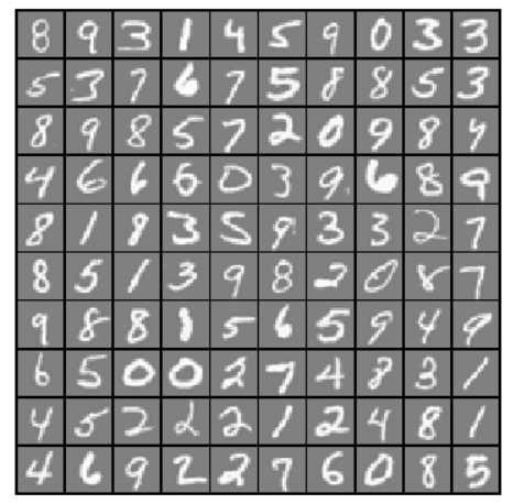
数据可视化
跟ex3几乎一模一样:
load('ex4data1.mat');
m = size(X, 1);

% Randomly select 100 data points to display
sel = randperm(size(X, 1));
sel = sel(1:100);
displayData(X(sel, :));
function [h, display_array] = displayData(X, example_width)
%DISPLAYDATA Display 2D data in a nice grid
%   [h, display_array] = DISPLAYDATA(X, example_width) displays 2D data
%   stored in X in a nice grid. It returns the figure handle h and the
%   displayed array if requested.

% Set example_width automatically if not passed in
if ~exist('example_width', 'var') || isempty(example_width)
    example_width = round(sqrt(size(X, 2)));
end

% Gray Image
colormap(gray);

% Compute rows, cols
[m n] = size(X);
example_height = (n / example_width);

% Compute number of items to display
display_rows = floor(sqrt(m));
display_cols = ceil(m / display_rows);

% Between images padding
pad = 1;

% Setup blank display
display_array = - ones(pad + display_rows * (example_height + pad), ...

                       pad + display_cols * (example_width + pad));

% Copy each example into a patch on the display array
curr_ex = 1;
for j = 1:display_rows
    for i = 1:display_cols
        if curr_ex > m,
            break;
        end
        % Copy the patch

        % Get the max value of the patch
        max_val = max(abs(X(curr_ex, :)));
        display_array(pad + (j - 1) * (example_height + pad) + (1:example_height), ...
                      pad + (i - 1) * (example_width + pad) + (1:example_width)) = ...
                        reshape(X(curr_ex, :), example_height, example_width) / max_val;
        curr_ex = curr_ex + 1;
    end
    if curr_ex > m,
        break;
    end
end

% Display Image
h = imagesc(display_array, [-1 1]);

% Do not show axis
axis image off

drawnow;

end
代价-梯度函数
进行一次向前传播得到代价函数值,再通过一次反向传播得到梯度,向量化推导见这篇博客,代码如下:
function [J grad] = nnCostFunction(nn_params, ...

                                   input_layer_size, ...

                                   hidden_layer_size, ...

                                   num_labels, ...

                                   X, y, lambda)
%NNCOSTFUNCTION Implements the neural network cost function for a two layer
%neural network which performs classification
%   [J grad] = NNCOSTFUNCTON(nn_params, hidden_layer_size, num_labels, ...

%   X, y, lambda) computes the cost and gradient of the neural network. The
%   parameters for the neural network are "unrolled" into the vector
%   nn_params and need to be converted back into the weight matrices.

%
%   The returned parameter grad should be a "unrolled" vector of the
%   partial derivatives of the neural network.

%

% Reshape nn_params back into the parameters Theta1 and Theta2, the weight matrices
% for our 2 layer neural network
Theta1 = reshape(nn_params(1:hidden_layer_size * (input_layer_size + 1)), ...

                 hidden_layer_size, (input_layer_size + 1));

Theta2 = reshape(nn_params((1 + (hidden_layer_size * (input_layer_size + 1))):end), ...

                 num_labels, (hidden_layer_size + 1));

% Setup some useful variables
m = size(X, 1);

% You need to return the following variables correctly
J = 0;
Theta1_grad = zeros(size(Theta1));
Theta2_grad = zeros(size(Theta2));

% ====================== YOUR CODE HERE ======================
% Instructions: You should complete the code by working through the
%               following parts.

%
% Part 1: Feedforward the neural network and return the cost in the
%         variable J. After implementing Part 1, you can verify that your
%         cost function computation is correct by verifying the cost
%         computed in ex4.m
%
% Part 2: Implement the backpropagation algorithm to compute the gradients
%         Theta1_grad and Theta2_grad. You should return the partial derivatives of
%         the cost function with respect to Theta1 and Theta2 in Theta1_grad and
%         Theta2_grad, respectively. After implementing Part 2, you can check
%         that your implementation is correct by running checkNNGradients
%
%         Note: The vector y passed into the function is a vector of labels
%               containing values from 1..K. You need to map this vector into a
%               binary vector of 1's and 0's to be used with the neural network
%               cost function.

%
%         Hint: We recommend implementing backpropagation using a for-loop
%               over the training examples if you are implementing it for the
%               first time.

%
% Part 3: Implement regularization with the cost function and gradients.

%
%         Hint: You can implement this around the code for
%               backpropagation. That is, you can compute the gradients for
%               the regularization separately and then add them to Theta1_grad
%               and Theta2_grad from Part 2.

%
target=zeros(m,num_labels);
for i=1:m
    target(i,y(i))=1;
end

X=[ones(m,1),X];
a2=sigmoid(X*Theta1');
a2=[ones(m,1),a2];
a3=sigmoid(a2*Theta2');

tmp=target.*log(a3)+(1.-target).*log(1-a3);
J=sum(sum(tmp));
J=-J/m;
J=J+(lambda/(2*m))*(sum(sum(Theta1.^2))-sum(Theta1(:,1).^2)+sum(sum(Theta2.^2))-sum(Theta2(:,1).^2));%记得减掉偏置项的参数

delta3=(a3-target)';
Theta2_grad=delta3*a2/m;
delta2=Theta2'*delta3.*a2'.*(1-a2');%别sigmoid(a2')
delta2=delta2(2:end,:);
Theta1_grad=delta2*X/m;

tmp1=Theta1_grad(:,1);
tmp2=Theta2_grad(:,1);
Theta1_grad=Theta1_grad+(lambda/m).*Theta1;
Theta1_grad(:,1)=tmp1;
Theta2_grad=Theta2_grad+(lambda/m).*Theta2;
Theta2_grad(:,1)=tmp2;

% -------------------------------------------------------------

% =========================================================================

% Unroll gradients
grad = [Theta1_grad(:) ; Theta2_grad(:)];

end
注意,为了能调用 fmincg这里用到了矩阵展开与复原的技巧,把矩阵转化为列向量这样才满足该函数的参数要求。
除了矩阵展开与复原,反向传播相对复杂,为了确保我们计算出的梯度正确,我们可以使用梯度检验来验证反向传播算出的梯度值。这里吴恩达直接直接提供了检查函数:
function checkNNGradients(lambda)
%CHECKNNGRADIENTS Creates a small neural network to check the
%backpropagation gradients
%   CHECKNNGRADIENTS(lambda) Creates a small neural network to check the
%   backpropagation gradients, it will output the analytical gradients
%   produced by your backprop code and the numerical gradients (computed
%   using computeNumericalGradient). These two gradient computations should
%   result in very similar values.

%

if ~exist('lambda', 'var') || isempty(lambda)
    lambda = 0;
end

input_layer_size = 3;
hidden_layer_size = 5;
num_labels = 3;
m = 5;

% We generate some 'random' test data
Theta1 = debugInitializeWeights(hidden_layer_size, input_layer_size);
Theta2 = debugInitializeWeights(num_labels, hidden_layer_size);
% Reusing debugInitializeWeights to generate X
X  = debugInitializeWeights(m, input_layer_size - 1);
y  = 1 + mod(1:m, num_labels)';

% Unroll parameters
nn_params = [Theta1(:) ; Theta2(:)];

% Short hand for cost function
costFunc = @(p) nnCostFunction(p, input_layer_size, hidden_layer_size, ...

                               num_labels, X, y, lambda);

[cost, grad] = costFunc(nn_params);
numgrad = computeNumericalGradient(costFunc, nn_params);

% Visually examine the two gradient computations.  The two columns
% you get should be very similar.

disp([numgrad grad]);
fprintf(['The above two columns you get should be very similar.\n' ...

         '(Left-Your Numerical Gradient, Right-Analytical Gradient)\n\n']);

% Evaluate the norm of the difference between two solutions.

% If you have a correct implementation, and assuming you used EPSILON = 0.0001
% in computeNumericalGradient.m, then diff below should be less than 1e-9
diff = norm(numgrad-grad)/norm(numgrad+grad);

fprintf(['If your backpropagation implementation is correct, then \n' ...

         'the relative difference will be small (less than 1e-9). \n' ...

         '\nRelative Difference: %g\n'], diff);

end
fmincg求解
有了代价-梯度函数,我们就可以开始求解了,设定好选项与正则系数λ \lambda λ,传入初始参数(记得用随机初始化)就可以等待函数返回是代价函数值最小的参数了。
options = optimset('MaxIter', 50);
lambda = 1;

% Create "short hand" for the cost function to be minimized
costFunction = @(p) nnCostFunction(p, input_layer_size, hidden_layer_size, num_labels, X, y, lambda);

% Now, costFunction is a function that takes in only one argument (the
% neural network parameters)
[nn_params, ~] = fmincg(costFunction, initial_nn_params, options);
预测
预测其实就是做一次向前传播再取最大值索引,不过要记得 fmincg找到的参数仍是展开的列向量,要使用的话需要复原。
% Obtain Theta1 and Theta2 back from nn_params
Theta1 = reshape(nn_params(1:hidden_layer_size * (input_layer_size + 1)), hidden_layer_size, (input_layer_size + 1));
Theta2 = reshape(nn_params((1 + (hidden_layer_size * (input_layer_size + 1))):end), num_labels, (hidden_layer_size + 1));

pred = predict(Theta1, Theta2, X);
fprintf('\nTraining Set Accuracy: %f\n', mean(double(pred == y)) * 100);
吴恩达提供了 predict.m,但我在ex3写的同样可以使用,那我肯定贴我的:
function p = predict(Theta1, Theta2, X)
%PREDICT Predict the label of an input given a trained neural network
%   p = PREDICT(Theta1, Theta2, X) outputs the predicted label of X given the
%   trained weights of a neural network (Theta1, Theta2)

% Useful values
m = size(X, 1);
num_labels = size(Theta2, 1);

% You need to return the following variables correctly
p = zeros(size(X, 1), 1);

% ====================== YOUR CODE HERE ======================
% Instructions: Complete the following code to make predictions using
%               your learned neural network. You should set p to a
%               vector containing labels between 1 to num_labels.

%
% Hint: The max function might come in useful. In particular, the max
%       function can also return the index of the max element, for more
%       information see 'help max'. If your examples are in rows, then, you
%       can use max(A, [], 2) to obtain the max for each row.

%

X=[ones(m,1) X];
tmp=sigmoid(X*Theta1');
tmp=[ones(m,1) tmp];
[~,p]=max(sigmoid(tmp*Theta2'),[],2);

% =========================================================================

end
对训练集的准确率为95.48 % 95.48\%9 5 .4 8 %。
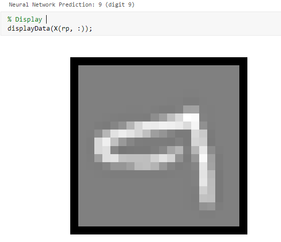
如果你想获得更好的体验,可以用下面的代码抽出一张随机图,由神经网络输出它的识别结果,同时下面打印出对应的手写数字图:
%  Randomly permute examples
rp = randi(m);
% Predict
pred = predict(Theta1, Theta2, X(rp,:));
fprintf('\nNeural Network Prediction: %d (digit %d)\n', pred, mod(pred, 10));
% Display
displayData(X(rp, :));
Original: https://blog.csdn.net/ShadyPi/article/details/122675355
Author: ShadyPi
Title: 机器学习:使用matlab实现神经网络解决数字识别(多元分类)问题
原创文章受到原创版权保护。转载请注明出处:https://www.johngo689.com/666040/
转载文章受原作者版权保护。转载请注明原作者出处!