吴恩达机器学习(五)逻辑回归练习-二分类练习

1、基础内容

（1）公式总结:

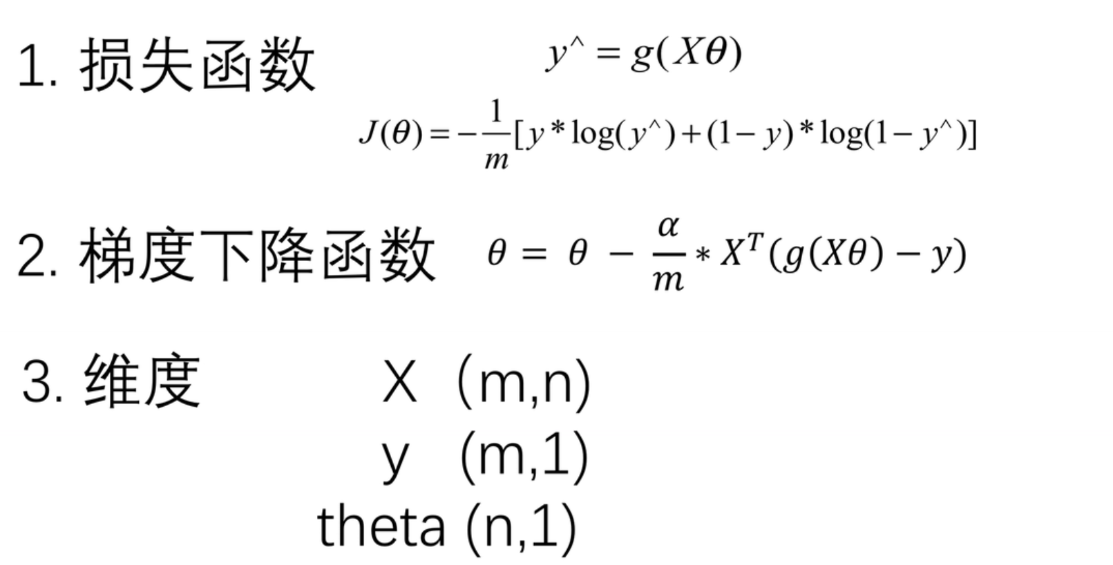
; （2）内容回归:

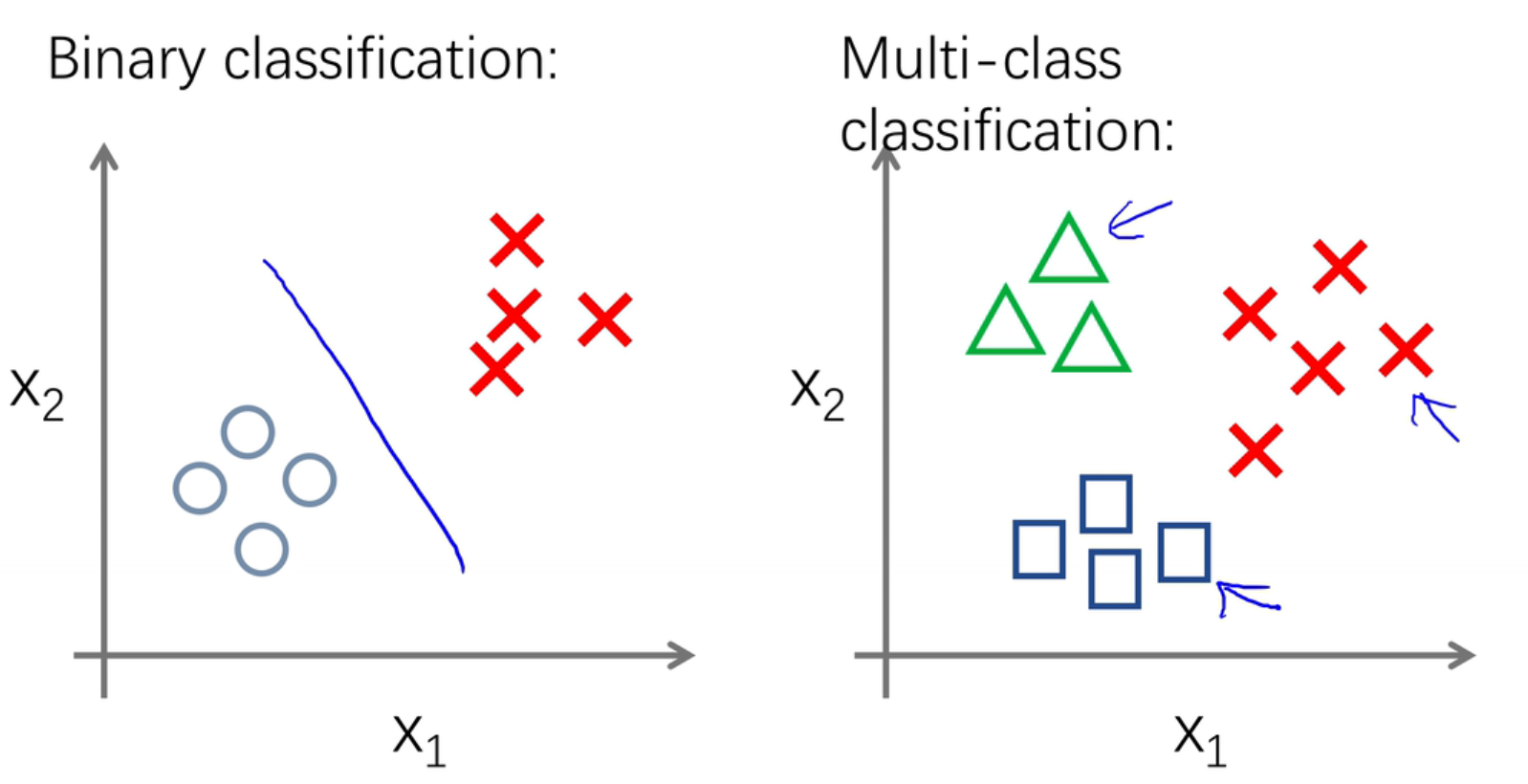
逻辑回归主要是进行二分类和多分类。

对于线性回归模型，我们定义的代价函数是所有模型误差的平方和。理论上来说，我们也可以对逻辑回归模型沿用这个定义，但是问题在于，当我们将h θ ( x ) {h_\theta}(x)h θ​(x )带入到这样定义了的代价函数中时，我们得到的代价函数将是一个非凸函数（ non-convexfunction）。

这意味着我们的代价函数有许多局部最小值，这将影响梯度下降算法寻找全局最小值。

线性回归的代价函数为：J ( θ ) = 1 m ∑ i = 1 m 1 2 ( h θ ( x ( i ) ) − y ( i ) ) 2 J\left( \theta \right)=\frac{1}{m}\sum\limits_{i=1}^{m}{\frac{1}{2}{{\left( {h_\theta}\left({x}^{\left( i \right)} \right)-{y}^{\left( i \right)} \right)}^{2}}}J (θ)=m 1 ​i =1 ∑m ​2 1 ​(h θ​(x (i ))−y (i ))2 。
我们重新定义逻辑回归的代价函数为：J ( θ ) = 1 m ∑ i = 1 m C o s t ( h θ ( x ( i ) ) , y ( i ) ) J\left( \theta \right)=\frac{1}{m}\sum\limits_{i=1}^{m}{{Cost}\left( {h_\theta}\left( {x}^{\left( i \right)} \right),{y}^{\left( i \right)} \right)}J (θ)=m 1 ​i =1 ∑m ​C o s t (h θ​(x (i )),y (i ))，其中

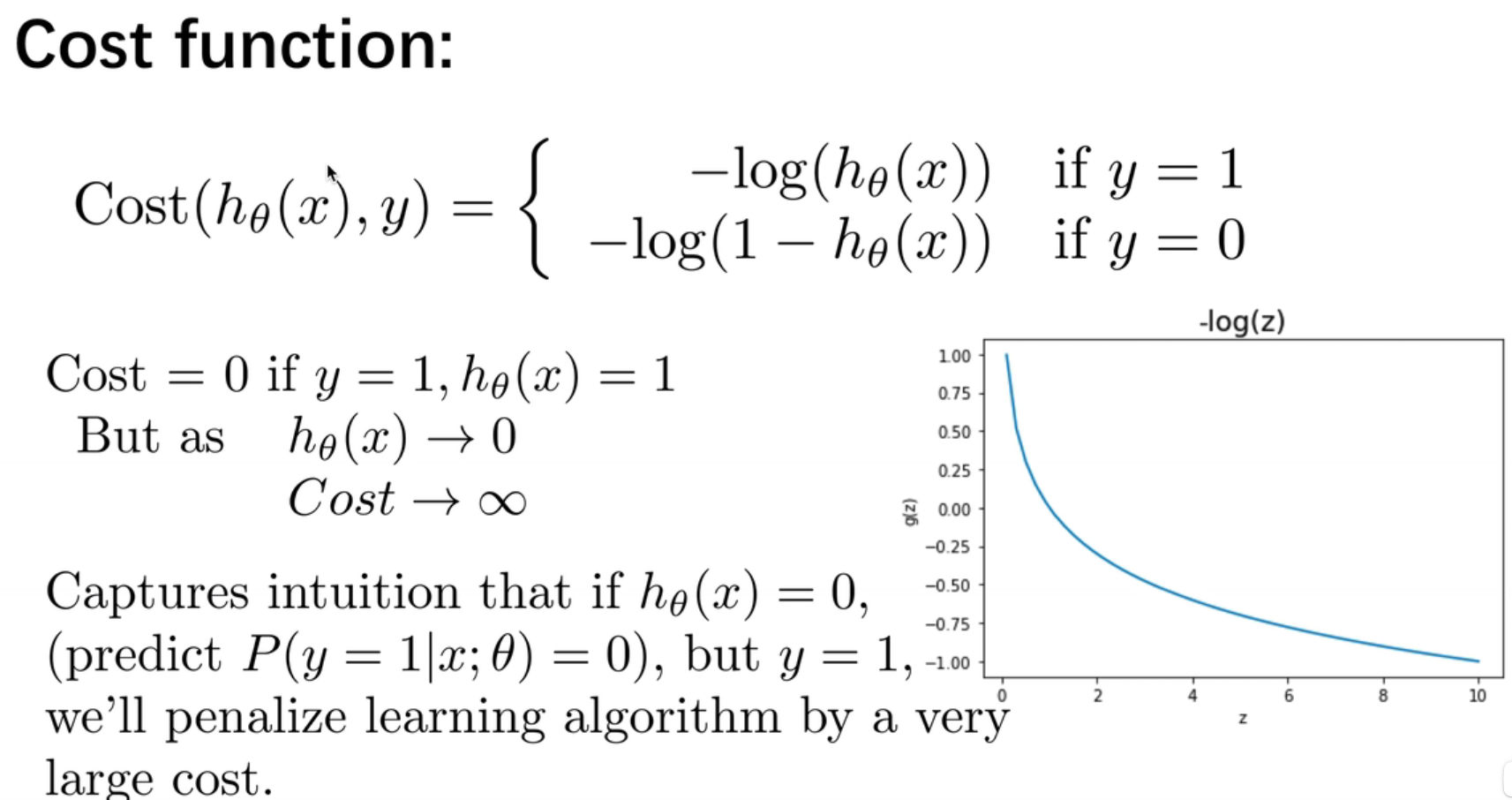
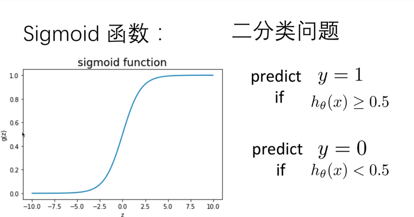
h θ ( x ) {h_\theta}\left( x \right)h θ​(x )与 C o s t ( h θ ( x ) , y ) Cost\left( {h_\theta}\left( x \right),y \right)C o s t (h θ​(x ),y )之间的关系如下图所示：

这样构建的C o s t ( h θ ( x ) , y ) Cost\left( {h_\theta}\left( x \right),y \right)C o s t (h θ​(x ),y )函数的特点是：当实际的 y = 1 y=1 y =1 且h θ ( x ) {h_\theta}\left( x \right)h θ​(x )也为 1 时误差为 0，当 y = 1 y=1 y =1 但h θ ( x ) {h_\theta}\left( x \right)h θ​(x )不为1时误差随着h θ ( x ) {h_\theta}\left( x \right)h θ​(x )变小而变大；当实际的 y = 0 y=0 y =0 且h θ ( x ) {h_\theta}\left( x \right)h θ​(x )也为 0 时代价为 0，当y = 0 y=0 y =0 但h θ ( x ) {h_\theta}\left( x \right)h θ​(x )不为 0时误差随着 h θ ( x ) {h_\theta}\left( x \right)h θ​(x )的变大而变大。
将构建的 C o s t ( h θ ( x ) , y ) Cost\left( {h_\theta}\left( x \right),y \right)C o s t (h θ​(x ),y )简化如下：
C o s t ( h θ ( x ) , y ) = − y × l o g ( h θ ( x ) ) − ( 1 − y ) × l o g ( 1 − h θ ( x ) ) Cost\left( {h_\theta}\left( x \right),y \right)=-y\times log\left( {h_\theta}\left( x \right) \right)-(1-y)\times log\left( 1-{h_\theta}\left( x \right) \right)C o s t (h θ​(x ),y )=−y ×l o g (h θ​(x ))−(1 −y )×l o g (1 −h θ​(x ))
带入代价函数得到：
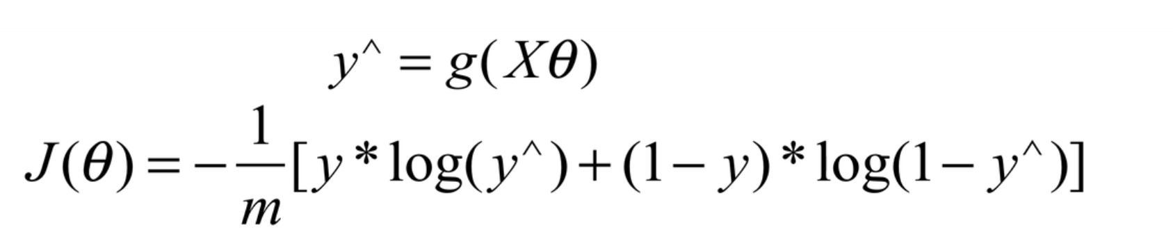
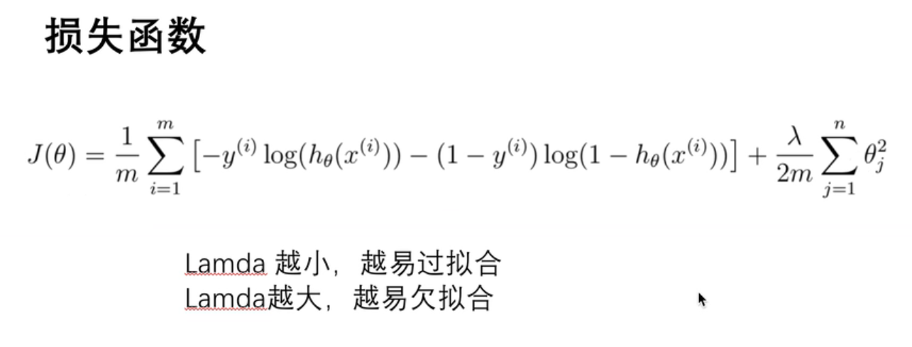
J ( θ ) = 1 m ∑ i = 1 m [ − y ( i ) log ⁡ ( h θ ( x ( i ) ) ) − ( 1 − y ( i ) ) log ⁡ ( 1 − h θ ( x ( i ) ) ) ] J\left( \theta \right)=\frac{1}{m}\sum\limits_{i=1}^{m}{[-{{y}^{(i)}}\log \left( {h_\theta}\left( {{x}^{(i)}} \right) \right)-\left( 1-{{y}^{(i)}} \right)\log \left( 1-{h_\theta}\left( {{x}^{(i)}} \right) \right)]}J (θ)=m 1 ​i =1 ∑m ​[−y (i )lo g (h θ​(x (i )))−(1 −y (i ))lo g (1 −h θ​(x (i )))]
即：J ( θ ) = − 1 m ∑ i = 1 m [ y ( i ) log ⁡ ( h θ ( x ( i ) ) ) + ( 1 − y ( i ) ) log ⁡ ( 1 − h θ ( x ( i ) ) ) ] J\left( \theta \right)=-\frac{1}{m}\sum\limits_{i=1}^{m}{[{{y}^{(i)}}\log \left( {h_\theta}\left( {{x}^{(i)}} \right) \right)+\left( 1-{{y}^{(i)}} \right)\log \left( 1-{h_\theta}\left( {{x}^{(i)}} \right) \right)]}J (θ)=−m 1 ​i =1 ∑m ​[y (i )lo g (h θ​(x (i )))+(1 −y (i ))lo g (1 −h θ​(x (i )))]

进行向量化表示;

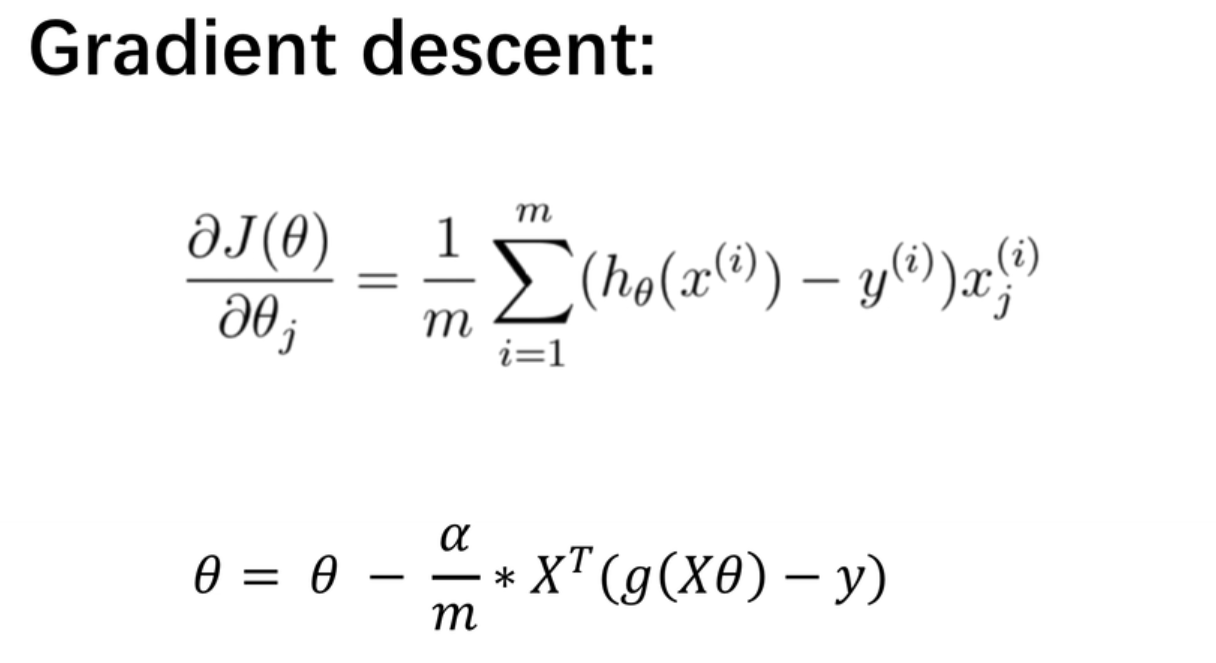
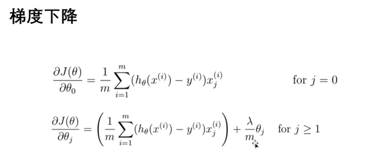
梯度下降和线性回归思路一样:

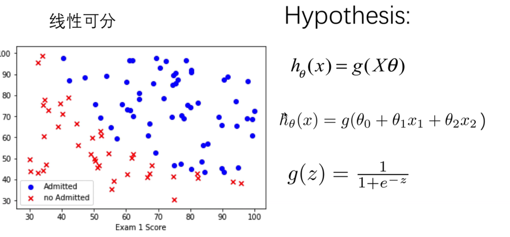
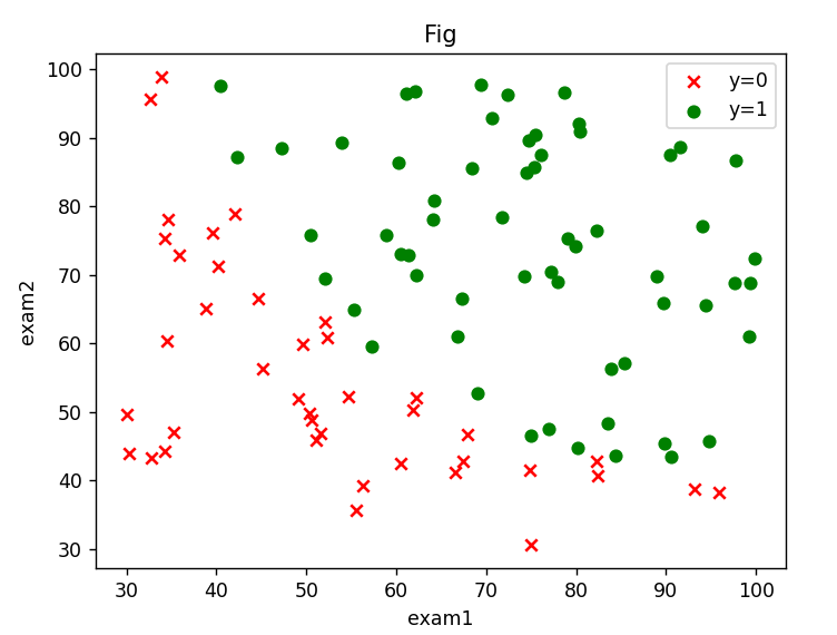
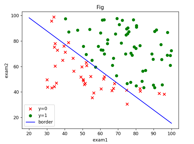
2、二分类案例(线性可分)___依据两次测试的成绩，预测是否被大学录取

（1）读取数据、绘制图像

"""
  二分类案例:
  依据两次测试的成绩，预测是否被大学录取
"""
import numpy as np
import pandas as pd
import matplotlib.pyplot as plt

df = pd.read_csv('ex2data1.txt',header=None,names=['exam1','exam2','accepted'])
print(df.head())

fig,ax = plt.subplots()
ax.scatter(df[df['accepted'] == 0]['exam1'],df[df['accepted'] == 0]['exam2'],c = 'red',marker='x' ,label='y=0')
ax.scatter(df[df['accepted'] == 1]['exam1'],df[df['accepted'] == 1]['exam2'],c = 'green',marker='o',label='y=1' )
ax.legend()
ax.set(xlabel='exam1',ylabel='exam2',title='Fig')
plt.show()

可以看出一个二分类问题。

(2)计算theta_final

def getX_y(df):

    df.insert(0,'const',1)

    X = df.iloc[:,0:-1]
    y = df.iloc[:, -1]

    X = X.values
    y = y.values
    y = y.reshape(len(y),1)
    return X,y

X,y = getX_y(df)

def sigmod(z):
    return 1 / (1 + np.exp(-z))

def costFunction(X, y, theta):
    A = sigmod(X @ theta)
    first = y * np.log(A)
    second = (1 - y) * np.log(1 - A)
    return -np.sum(first + second) / len(y)

def gradientDescent(X, y, theta, alpha, iters):
    costs = []
    for i in range(iters):
        A = sigmod(X @ theta)
        theta = theta - (alpha * X.T @ (A - y)) / (len(y))
        cost = costFunction(X, y, theta)
        costs.append(cost)

        if i % 1000 == 0:
            print(cost)
    return theta, costs

alpha = 0.004
iters = 200000

theta = np.zeros((3,1))

theta_final,costs = gradientDescent(X,y,theta,alpha,iters)
print(theta_final)

（3）计算预测准确率，绘制决策边界

def predict(X, theta):
    p = sigmod(X @ theta)
    return [1 if x >= 0.5 else 0 for x in p]

y_ = np.array(predict(X,theta_final))
y_pre = y_.reshape(len(y_),1)
acc = np.mean(y_pre == y)
print(acc)

x = np.linspace(20,100,100)
f = - theta_final[0,0] / theta_final[2,0] - theta_final[1,0] / theta_final[2,0] * x

fig,ax = plt.subplots()
ax.scatter(df[df['accepted'] == 0]['exam1'],df[df['accepted'] == 0]['exam2'],c = 'red',marker='x' ,label='y=0')
ax.scatter(df[df['accepted'] == 1]['exam1'],df[df['accepted'] == 1]['exam2'],c = 'green',marker='o',label='y=1' )
ax.plot(x,f,c = 'blue',label='border' )
ax.legend()
ax.set(xlabel='exam1',ylabel='exam2',title='Fig')
plt.show()

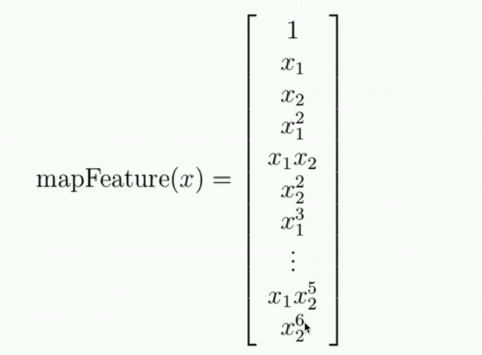
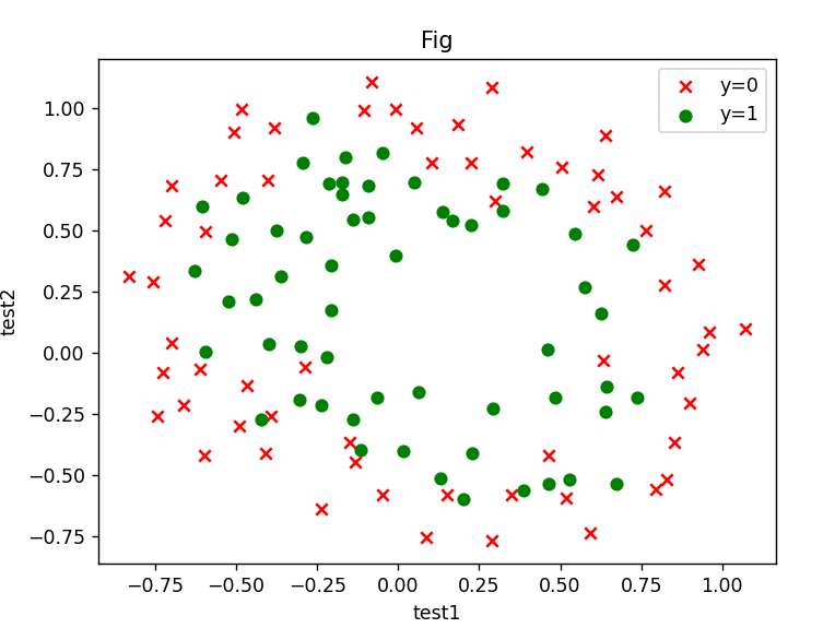
3、二分类案例(线性不可分)___依据两次测试的成绩，决定芯片要被抛弃还是接受

没有办法用一条直线进行切分。

需要特征映射:

为了防止过拟合，需要加上正则项：


(1)读取原始数据，画图

"""
  逻辑回归练习（线性不可分）:
    决定芯片要被抛弃还是接受
    数据集： 芯片在两次测试中的测试结果
"""
import numpy as np
import pandas as pd
import matplotlib.pyplot as plt

df = pd.read_csv('ex2data2.txt',header=None,names=['test1','test2','accepted'])
print(df.head())

fig,ax = plt.subplots()
ax.scatter(df[df['accepted'] == 0]['test1'],df[df['accepted'] == 0]['test2'],c = 'red',marker='x' ,label='y=0')
ax.scatter(df[df['accepted'] == 1]['test1'],df[df['accepted'] == 1]['test2'],c = 'green',marker='o',label='y=1' )
ax.legend()
ax.set(xlabel='test1',ylabel='test2',title='Fig')
plt.show()

(2)使用特征映射，定义函数计算theta

def feature_mapping(x1, x2, power):
    data = {}
    for i in np.arange(power + 1):
        for j in np.arange(i + 1):
            data['F{}{}'.format(i - j, j)] = np.power(x1, i - j) * np.power(x2, j)
    return pd.DataFrame(data)
x1 = df['test1']
x2 = df['test2']

mdf = feature_mapping(x1,x2,6)

y = df.iloc[:, -1]

X = mdf.values
y = y.values
y = y.reshape(len(y),1)

def sigmod(z):
    return 1 / (1 + np.exp(-z))

def costFunction(X, y, theta, lamda):
    A = sigmod(X @ theta)
    first = y * np.log(A)
    second = (1 - y) * np.log(1 - A)

    reg = np.sum( np.power(theta[1:],2) ) * (lamda / (2 * len(y)) )
    return -np.sum(first + second) / len(y) + reg

def gradientDescent(X, y, theta, alpha, iters, lamda):
    costs = []
    for i in range(iters):
        reg = theta[1:] * (lamda / len(y))
        reg = np.insert(reg, 0, values=0, axis=0)

        A = sigmod(X @ theta)
        theta = theta - (alpha * X.T @ (A - y)) / (len(y)) - alpha * reg
        cost = costFunction(X, y, theta, lamda)
        costs.append(cost)
        if i % 1000 == 0:
            print(cost)
    return theta, costs

alpha = 0.001
iters = 20000

lamda = 0.0001
theta = np.zeros((28,1))

theta_final,costs = gradientDescent(X,y,theta,alpha,iters,lamda)
print(theta_final)

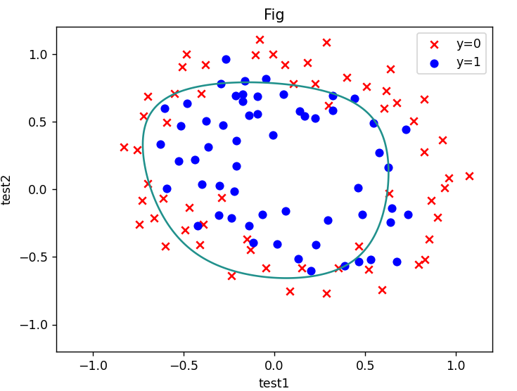
(3)计算预测准确率，画出决策边界

def predict(X, theta):
    p = sigmod(X @ theta)

    return [1 if x >= 0.5 else 0 for x in p]

y_ = np.array(predict(X,theta_final))
y_pre = y_.reshape(len(y_),1)
acc = np.mean(y_pre == y)
print(acc)

x = np.linspace(-1.2,1.2,200)
xx,yy = np.meshgrid(x,x)
print(xx.shape)
z = feature_mapping(xx.ravel(),yy.ravel(),6).values
zz = z @ theta_final
zz = zz.reshape(200,200)

fig,ax = plt.subplots()
ax.scatter(df[df['accepted'] == 0]['test1'],df[df['accepted'] == 0]['test2'],c = 'red',marker='x' ,label='y=0')
ax.scatter(df[df['accepted'] == 1]['test1'],df[df['accepted'] == 1]['test2'],c = 'blue',marker='o',label='y=1' )
ax.legend()
ax.set(xlabel='test1',ylabel='test2',title='Fig')
plt.contour(xx,yy,zz,0)
plt.show()

Original: https://blog.csdn.net/qq_44665283/article/details/123028916
Author: undo_try
Title: 吴恩达机器学习(五)逻辑回归练习-二分类练习