


文章目录
- 前言
- 支持模型(点击跳转到训练自己数据集教程页)
- 环境搭建
- 数据集准备
* - 1. 标签文件制作
- 2. 数据集划分
- 3. 数据集信息文件制作
- 配置文件解释
- 如何训练
- 模型评估
- 添加新的模型组件
* - 添加新的主干网络Backbone
- 添加新的颈部Neck
- 添加新的头部Head
- 添加新的损失函数Loss
- 类别激活图可视化
- 学习率策略可视化
- 预训练权重
; 前言
项目地址:https://github.com/Fafa-DL/Awesome-Backbones
无法访问GitHub:公众号【啥都会一点的研究生】-课程资源-我的项目-00
视频教程:https://www.bilibili.com/video/BV1SY411P7Nd
本文章用于照顾无法进入Github的同学~
初衷:
- 帮助大家从简单的LeNet网络到Transformer网络进行复现学习;
- 帮助提高阅读工程代码的能力;
- 帮助进行网络对比/炼丹/发paper
支持模型(点击跳转到训练自己数据集教程页)
- LeNet5
- AlexNet
- VGG
- DenseNet
- ResNet
- ResNeXt
- SEResNet
- SEResNeXt
- RegNet
- MobileNetV2
- MobileNetV3
- ShuffleNetV1
- ShuffleNetV2
- EfficientNet
- RepVGG
- Res2Net
- ConvNeXt
- HRNet
- ConvMixer
- CSPNet
- Swin-Transformer
- Vision-Transformer
- Transformer-in-Transformer
- MLP-Mixer
- DeiT
- Conformer
- T2T-ViT
- Twins
- PoolFormer
- VAN
环境搭建
- 建议使用Anaconda进行环境管理,创建环境命令如下
conda create -n [name] python=3.6 其中[name]改成自己的环境名,如[name]->torch,conda create -n torch python=3.6
- 我的测试环境如下
torch==1.7.1
torchvision==0.8.2
scipy==1.4.1
numpy==1.19.2
matplotlib==3.2.1
opencv_python==3.4.1.15
tqdm==4.62.3
Pillow==8.4.0
h5py==3.1.0
terminaltables==3.1.0
packaging==21.3
- 首先安装Pytorch。建议版本和我一致,进入Pytorch官网,点击
install previous versions of PyTorch,以1.7.1为例,官网给出的安装如下,选择合适的cuda版本
CUDA 11.0
pip install torch==1.7.1+cu110 torchvision==0.8.2+cu110 torchaudio==0.7.2 -f https://download.pytorch.org/whl/torch_stable.html

CUDA 10.2
pip install torch==1.7.1 torchvision==0.8.2 torchaudio==0.7.2

CUDA 10.1
pip install torch==1.7.1+cu101 torchvision==0.8.2+cu101 torchaudio==0.7.2 -f https://download.pytorch.org/whl/torch_stable.html

CUDA 9.2
pip install torch==1.7.1+cu92 torchvision==0.8.2+cu92 torchaudio==0.7.2 -f https://download.pytorch.org/whl/torch_stable.html

CPU only
pip install torch==1.7.1+cpu torchvision==0.8.2+cpu torchaudio==0.7.2 -f https://download.pytorch.org/whl/torch_stable.html
- 安装完Pytorch后,再运行
pip install -r requirements.txt
数据集准备
1. 标签文件制作
- 本次演示以花卉数据集为例,目录结构如下:
├─flower_photos
│  ├─daisy
│  │      100080576_f52e8ee070_n.jpg
│  │      10140303196_b88d3d6cec.jpg
│  │      ...

│  ├─dandelion
│  │      10043234166_e6dd915111_n.jpg
│  │      10200780773_c6051a7d71_n.jpg
│  │      ...

│  ├─roses
│  │      10090824183_d02c613f10_m.jpg
│  │      102501987_3cdb8e5394_n.jpg
│  │      ...

│  ├─sunflowers
│  │      1008566138_6927679c8a.jpg
│  │      1022552002_2b93faf9e7_n.jpg
│  │      ...

│  └─tulips
│  │      100930342_92e8746431_n.jpg
│  │      10094729603_eeca3f2cb6.jpg
│  │      ...
- 在
Awesome-Backbones/datas/中创建标签文件annotations.txt,按行将类别名 索引写入文件;
daisy 0
dandelion 1
roses 2
sunflowers 3
tulips 4
2. 数据集划分
- 打开
Awesome-Backbones/tools/split_data.py - 修改
原始数据集路径以及划分后的保存路径,强烈建议划分后的保存路径datasets不要改动,在下一步都是默认基于文件夹进行操作
init_dataset = 'A:/flower_photos'
new_dataset = 'A:/Awesome-Backbones/datasets'
- 在
Awesome-Backbones/下打开终端输入命令:
python tools/split_data.py
- 得到划分后的数据集格式如下:
├─...

├─datasets
│  ├─test
│  │  ├─daisy
│  │  ├─dandelion
│  │  ├─roses
│  │  ├─sunflowers
│  │  └─tulips
│  └─train
│      ├─daisy
│      ├─dandelion
│      ├─roses
│      ├─sunflowers
│      └─tulips
├─...
3. 数据集信息文件制作
- 确保划分后的数据集是在
Awesome-Backbones/datasets下,若不在则在get_annotation.py下修改数据集路径;
datasets_path = '你的数据集路径'
- 在
Awesome-Backbones/下打开终端输入命令:
python tools/get_annotation.py
- 在
Awesome-Backbones/datas下得到生成的数据集信息文件train.txt与test.txt
配置文件解释
- 每个模型均对应有各自的配置文件,保存在
Awesome-Backbones/models下 - Model
'''
由backbone、neck、head、head.loss构成一个完整模型;

type与相应结构对应,其后紧接搭建该结构所需的参数,每个配置文件均已设置好;

配置文件中的 type 不是构造时的参数,而是类名。

需修改的地方:num_classes修改为对应数量,如花卉数据集为五类,则num_classes=5

注意如果类别数小于5则此时默认top5准确率为100%
'''
model_cfg = dict(
    backbone=dict(
        type='ResNet',
        depth=50,
        num_stages=4,
        out_indices=(3, ),
        frozen_stages=-1,
        style='pytorch'),
    neck=dict(type='GlobalAveragePooling'),
    head=dict(
        type='LinearClsHead',
        num_classes=1000,
        in_channels=2048,
        loss=dict(type='CrossEntropyLoss', loss_weight=1.0),
        topk=(1, 5),
    ))
- Datasets
'''
该部分对应构建训练/测试时的Datasets,使用torchvision.transforms进行预处理;

size=224为最终处理后,喂入网络的图像尺寸;

Normalize对应归一化,默认使用ImageNet数据集均值与方差,若你有自己数据集的参数,可以选择覆盖。
'''
train_pipeline = (
    dict(type='RandomResizedCrop', size=224),
    dict(type='RandomHorizontalFlip', p=0.5),
    dict(type='ToTensor'),
    dict(type='Normalize', mean=[0.485, 0.456, 0.406], std=[0.229, 0.224, 0.225]),
    dict(type='RandomErasing',p=0.2,ratio=(0.02,1/3)),
)
val_pipeline = (
    dict(type='Resize', size=256),
    dict(type='CenterCrop', size=224),
    dict(type='ToTensor'),
    dict(type='Normalize', mean=[0.485, 0.456, 0.406], std=[0.229, 0.224, 0.225])
)
- Train/Test
'''
该部分对应训练/测试所需参数;

batch_size                 : 根据自己设备进行调整,建议为2的倍数
num_workers            : Dataloader中加载数据的线程数,根据自己设备调整
pretrained_flag          : 若使用预训练权重,则设置为True
pretrained_weights    : 权重路径
freeze_flag                : 若冻结某部分训练,则设置为True
freeze_layers              :可选冻结的有backbone, neck, head
epoches                    : 最大迭代周期

ckpt : 评估模型所需的权重文件
注意如果类别数小于5则此时默认top5准确率为100%
其余参数均不用改动
'''
data_cfg = dict(
    batch_size = 32,
    num_workers = 4,
    train = dict(
        pretrained_flag = False,
        pretrained_weights = './datas/mobilenet_v3_small.pth',
        freeze_flag = False,
        freeze_layers = ('backbone',),
        epoches = 100,
    ),
    test=dict(
        ckpt = 'logs/20220202091725/Val_Epoch019-Loss0.215.pth',
        metrics = ['accuracy', 'precision', 'recall', 'f1_score', 'confusion'],
        metric_options = dict(
            topk = (1,5),
            thrs = None,
            average_mode='none'
    ))
)
- Optimizer
'''
训练时的优化器,与torch.optim对应

type : 'RMSprop'对应torch.optim.RMSprop,可在torch.optim查看
PyTorch支持Adadelta、Adagrad、Adam、AdamW、SparseAdam、Adamax、ASGD、SGD、Rprop、RMSprop、Optimizer、LBFGS
可以根据自己需求选择优化器

lr      : 初始学习率,可根据自己Batch Size调整
ckpt : 评估模型所需的权重文件

其余参数均不用改动
'''
optimizer_cfg = dict(
    type='RMSprop',
    lr=0.001,
    alpha=0.9,
    momentum=0.9,
    eps=0.0316,
    weight_decay=1e-5)
- Learning Rate
'''
学习率更新策略,各方法可在Awesome-Backbones/core/optimizers/lr_update.py查看

StepLrUpdater                    : 线性递减
CosineAnnealingLrUpdater : 余弦退火

by_epoch                : 是否每个Epoch更新学习率
warmup                  : 在正式使用学习率更新策略前先用warmup小学习率训练,可选constant, linear, exp
warmup_ratio          : 与Optimizer中的lr结合所选warmup方式进行学习率运算更新
warmup_by_epoch  : 作用与by_epoch类似,若为False,则为每一步(Batch)进行更新,否则每周期
warmup_iters          : warmup作用时长,warmup_by_epoch为True则代表周期,False则代表步数
'''
lr_config = dict(
    type='CosineAnnealingLrUpdater',
    by_epoch=False,
    min_lr_ratio=1e-2,
    warmup='linear',
    warmup_ratio=1e-3,
    warmup_iters=20,
    warmup_by_epoch=True)
如何训练
- 确认
Awesome-Backbones/datas/annotations.txt标签准备完毕 - 确认
Awesome-Backbones/datas/下train.txt与test.txt与annotations.txt对应 - 选择想要训练的模型,在
Awesome-Backbones/models/下找到对应配置文件 - 按照
配置文件解释修改参数 - 在
Awesome-Backbones打开终端运行
python tools/train.py models/mobilenet/mobilenet_v3_small.py
命令行:
python tools/train.py \
    ${CONFIG_FILE} \
    [--resume-from] \
    [--seed] \
    [--device] \
    [--gpu-id] \
    [--deterministic] \
所有参数的说明:
config:模型配置文件的路径。--resume-from:从中断处恢复训练,提供权重路径,务必注意正确的恢复方式是从Last_Epoch***.pth,如–resume-from logs/SwinTransformer/2022-02-08-08-27-41/Last_Epoch15.pth--seed:设置随机数种子,默认按照环境设置--device:设置GPU或CPU训练--gpu-id:指定GPU设备,默认为0(单卡基本均为0不用改动)--deterministic:多GPU训练相关,暂不用设置
模型评估
- 确认
Awesome-Backbones/datas/annotations.txt标签准备完毕 - 确认
Awesome-Backbones/datas/下test.txt与annotations.txt对应 - 在
Awesome-Backbones/models/下找到对应配置文件 - 按照
配置文件解释修改参数,主要修改权重路径 - 在
Awesome-Backbones打开终端运行
python tools/evaluation.py models/mobilenet/mobilenet_v3_small.py
- 单张图像测试,在
Awesome-Backbones打开终端运行
python tools/single_test.py datasets/test/dandelion/14283011_3e7452c5b2_n.jpg models/mobilenet/mobilenet_v3_small.py
参数说明:
img : 被测试的单张图像路径
config : 模型配置文件,需注意修改配置文件中 data_cfg->test->ckpt的权重路径,将使用该权重进行预测
--device : 推理所用设备,默认GPU
--save-path : 保存路径,默认不保存
添加新的模型组件
- 一个完整的模型由
Backbone、Neck、Head、Loss组成,在文件夹configs下可以找到 - 主干网络:通常是一个特征提取网络,例如 ResNet、MobileNet
- 颈部:用于连接主干网络和头部的组件,例如 GlobalAveragePooling
- 头部:用于执行特定任务的组件,例如分类和回归
- 损失:用于计算预测值与真实值偏差值
添加新的主干网络Backbone
以 ResNet_CIFAR 为例

ResNet_CIFAR 针对 CIFAR 32x32 的图像输入,将 ResNet 中 kernel_size=7, stride=2 的设置替换为 kernel_size=3, stride=1,并移除了 stem 层之后的 MaxPooling,以避免传递过小的特征图到残差块中。

它继承自 ResNet 并只修改了 stem 层。
- 创建一个新文件
configs/backbones/resnet_cifar.py。
import torch.nn as nn

from ..common import BaseModule
from .resnet import ResNet

class ResNet_CIFAR(ResNet):

    """ResNet backbone for CIFAR.

    (对这个主干网络的简短描述)

    Args:
        depth(int): Network depth, from {18, 34, 50, 101, 152}.

        ...

        (参数文档)
"""

    def __init__(self, depth, deep_stem=False, **kwargs):

        super(ResNet_CIFAR, self).__init__(depth, deep_stem=deep_stem **kwargs)

        assert not self.deep_stem, 'ResNet_CIFAR do not support deep_stem'

    def _make_stem_layer(self, in_channels, base_channels):

        self.conv1 = build_conv_layer(
            self.conv_cfg,
            in_channels,
            base_channels,
            kernel_size=3,
            stride=1,
            padding=1,
            bias=False)
        self.norm1_name, norm1 = build_norm_layer(
            self.norm_cfg, base_channels, postfix=1)
        self.add_module(self.norm1_name, norm1)
        self.relu = nn.ReLU(inplace=True)

    def forward(self, x):
        pass

    def init_weights(self, pretrained=None):
        pass

    def train(self, mode=True):
        pass
- 在
configs/backbones/__init__.py中导入新模块
...

from .resnet_cifar import ResNet_CIFAR

__all__ = [
    ..., 'ResNet_CIFAR'
]
- 在配置文件中使用新的主干网络
model_cfg = dict(
    backbone=dict(
        type='ResNet_CIFAR',
        depth=18,
        other_arg=xxx),
    ...
添加新的颈部Neck
以 GlobalAveragePooling 为例

要添加新的颈部组件,主要需要实现 forward 函数,该函数对主干网络的输出进行 一些操作并将结果传递到头部。
- 创建一个新文件
configs/necks/gap.py
import torch.nn as nn

class GlobalAveragePooling(nn.Module):

    def __init__(self):
        self.gap = nn.AdaptiveAvgPool2d((1, 1))

    def forward(self, inputs):

        outs = self.gap(inputs)
        outs = outs.view(inputs.size(0), -1)
        return outs
在configs/necks/__init__.py中导入新模块
...

from .gap import GlobalAveragePooling

__all__ = [
    ..., 'GlobalAveragePooling'
]
- 修改配置文件以使用新的颈部组件
model_cfg = dict(
    neck=dict(type='GlobalAveragePooling'),
)
添加新的头部Head
以 LinearClsHead 为例

要添加新的颈部组件,主要需要实现 forward 函数,该函数对主干网络的输出进行 一些操作并将结果传递到头部。
- 创建一个新文件
configs/heads/linear_head.py
from .cls_head import ClsHead

class LinearClsHead(ClsHead):

    def __init__(self,
              num_classes,
              in_channels,
              loss=dict(type='CrossEntropyLoss', loss_weight=1.0),
              topk=(1, )):
        super(LinearClsHead, self).__init__(loss=loss, topk=topk)
        self.in_channels = in_channels
        self.num_classes = num_classes

        if self.num_classes  0:
            raise ValueError(
                f'num_classes={num_classes} must be a positive integer')

        self._init_layers()

    def _init_layers(self):
        self.fc = nn.Linear(self.in_channels, self.num_classes)

    def init_weights(self):
        normal_init(self.fc, mean=0, std=0.01, bias=0)

    def forward_train(self, x, gt_label):
        cls_score = self.fc(x)
        losses = self.loss(cls_score, gt_label)
        return losses
在configs/heads/__init__.py中导入新模块
...

from .linear_head import LinearClsHead

__all__ = [
    ..., 'LinearClsHead'
]
- 修改配置文件以使用新的颈部组件,连同 GlobalAveragePooling 颈部组件,完整的模型配置如下:
model_cfg = dict(
    backbone=dict(
        type='ResNet',
        depth=50,
        num_stages=4,
        out_indices=(3, ),
        style='pytorch'),
    neck=dict(type='GlobalAveragePooling'),
    head=dict(
        type='LinearClsHead',
        num_classes=1000,
        in_channels=2048,
        loss=dict(type='CrossEntropyLoss', loss_weight=1.0),
        topk=(1, 5),
    ))
添加新的损失函数Loss
要添加新的损失函数,主要需要在损失函数模块中 forward 函数。另外,利用装饰器 weighted_loss 可以方便的实现对每个元素的损失进行加权平均。

假设我们要模拟从另一个分类模型生成的概率分布,需要添加 L1loss 来实现该目的。
- 创建一个新文件
configs/losses/l1_loss.py
import torch
import torch.nn as nn

from .utils import weighted_loss

@weighted_loss
def l1_loss(pred, target):
    assert pred.size() == target.size() and target.numel() > 0
    loss = torch.abs(pred - target)
    return loss

class L1Loss(nn.Module):

    def __init__(self, reduction='mean', loss_weight=1.0):
        super(L1Loss, self).__init__()
        self.reduction = reduction
        self.loss_weight = loss_weight

    def forward(self,
                pred,
                target,
                weight=None,
                avg_factor=None,
                reduction_override=None):
        assert reduction_override in (None, 'none', 'mean', 'sum')
        reduction = (
            reduction_override if reduction_override else self.reduction)
        loss = self.loss_weight * l1_loss(
            pred, target, weight, reduction=reduction, avg_factor=avg_factor)
        return loss
在configs/losses/__init__.py中导入新模块
...

from .l1_loss import L1Loss, l1_loss

__all__ = [
    ..., 'L1Loss', 'l1_loss'
]
- 修改配置文件中的
loss字段以使用新的损失函数
loss=dict(type='L1Loss', loss_weight=1.0))
类别激活图可视化
- 提供
tools/vis_cam.py工具来可视化类别激活图。请使用pip install grad-cam安装依赖,版本≥1.3.6 - 在
Awesome-Backbones/models/下找到对应配置文件 - 修改data_cfg中test的ckpt路径,改为训练完毕的权重
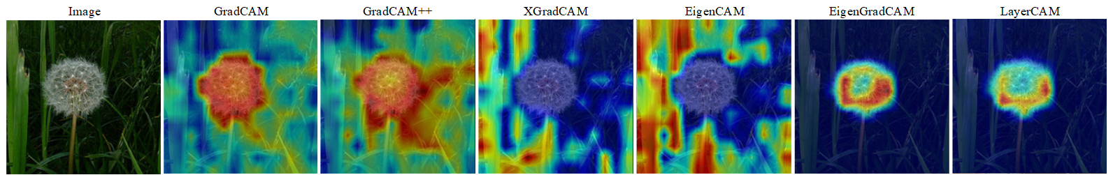
目前支持的方法有:
MethodWhat it doesGradCAM使用平均梯度对 2D 激活进行加权GradCAM++类似 GradCAM,但使用了二阶梯度XGradCAM类似 GradCAM,但通过归一化的激活对梯度进行了加权EigenCAM使用 2D 激活的第一主成分(无法区分类别,但效果似乎不错)EigenGradCAM类似 EigenCAM,但支持类别区分,使用了激活 * 梯度的第一主成分,看起来和 GradCAM 差不多,但是更干净LayerCAM使用正梯度对激活进行空间加权,对于浅层有更好的效果
命令行:
python tools/vis_cam.py \
    ${IMG} \
    ${CONFIG_FILE} \
    [--target-layers ${TARGET-LAYERS}] \
    [--preview-model] \
    [--method ${METHOD}] \
    [--target-category ${TARGET-CATEGORY}] \
    [--save-path ${SAVE_PATH}] \
    [--vit-like] \
    [--num-extra-tokens ${NUM-EXTRA-TOKENS}]
    [--aug_smooth] \
    [--eigen_smooth] \
    [--device ${DEVICE}] \
所有参数的说明:
img:目标图片路径。config:模型配置文件的路径。需注意修改配置文件中data_cfg->test->ckpt的权重路径,将使用该权重进行预测--target-layers:所查看的网络层名称,可输入一个或者多个网络层, 如果不设置,将使用最后一个block中的norm层。--preview-model:是否查看模型所有网络层。--method:类别激活图图可视化的方法,目前支持GradCAM,GradCAM++,XGradCAM,EigenCAM,EigenGradCAM,LayerCAM,不区分大小写。如果不设置,默认为GradCAM。--target-category:查看的目标类别,如果不设置,使用模型检测出来的类别做为目标类别。--save-path:保存的可视化图片的路径,默认不保存。--eigen-smooth:是否使用主成分降低噪音,默认不开启。--vit-like: 是否为ViT类似的 Transformer-based 网络--num-extra-tokens:ViT类网络的额外的 tokens 通道数,默认使用主干网络的num_extra_tokens。--aug-smooth:是否使用测试时增强--device:使用的计算设备,如果不设置,默认为’cpu’。
在指定 --target-layers 时,如果不知道模型有哪些网络层,可使用命令行添加 --preview-model 查看所有网络层名称;
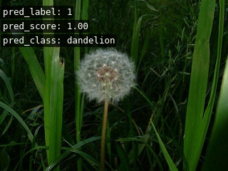
示例(CNN):
- 使用不同方法可视化
MobileNetV3,默认target-category为模型检测的结果,使用默认推导的target-layers。
python tools/vis_cam.py datasets/test/dandelion/14283011_3e7452c5b2_n.jpg models/mobilenet/mobilenet_v3_small.py
- 指定同一张图中不同类别的激活图效果图,给定类别索引即可
python tools/vis_cam.py datasets/test/dandelion/14283011_3e7452c5b2_n.jpg models/mobilenet/mobilenet_v3_small.py --target-category 1
- 使用
--eigen-smooth以及--aug-smooth获取更好的可视化效果。
python tools/vis_cam.py datasets/test/dandelion/14283011_3e7452c5b2_n.jpg models/mobilenet/mobilenet_v3_small.py --eigen-smooth --aug-smooth
示例(Transformer):
对于 Transformer-based 的网络,比如 ViT、T2T-ViT 和 Swin-Transformer,特征是被展平的。为了绘制 CAM 图,需要指定 --vit-like 选项,从而让被展平的特征恢复方形的特征图。
除了特征被展平之外,一些类 ViT 的网络还会添加额外的 tokens。比如 ViT 和 T2T-ViT 中添加了分类 token,DeiT 中还添加了蒸馏 token。在这些网络中,分类计算在最后一个注意力模块之后就已经完成了,分类得分也只和这些额外的 tokens 有关,与特征图无关,也就是说,分类得分对这些特征图的导数为 0。因此,我们不能使用最后一个注意力模块的输出作为 CAM 绘制的目标层。
另外,为了去除这些额外的 toekns 以获得特征图,我们需要知道这些额外 tokens 的数量。MMClassification 中几乎所有 Transformer-based 的网络都拥有 num_extra_tokens 属性。而如果你希望将此工具应用于新的,或者第三方的网络,而且该网络没有指定 num_extra_tokens 属性,那么可以使用 --num-extra-tokens 参数手动指定其数量。
- 对
Swin Transformer使用默认target-layers进行 CAM 可视化:
python tools/vis_cam.py datasets/test/dandelion/14283011_3e7452c5b2_n.jpg models/swin_transformer/tiny_224.py --vit-like
- 对
Vision Transformer(ViT)进行 CAM 可视化(经测试其实不加–target-layer即默认效果也差不多):
python tools/vis_cam.py datasets/test/dandelion/14283011_3e7452c5b2_n.jpg models/vision_transformer/vit_base_p16_224.py --vit-like --target-layers backbone.layers[-1].ln1
- 对
T2T-ViT进行 CAM 可视化:
python tools/vis_cam.py datasets/test/dandelion/14283011_3e7452c5b2_n.jpg models/t2t_vit/t2t_vit_t_14.py --vit-like --target-layers backbone.encoder[-1].ln1

学习率策略可视化
- 提供
tools/vis_lr.py工具来可视化学习率。
命令行:
python tools/vis_lr.py \
    ${CONFIG_FILE} \
    [--dataset-size ${Dataset_Size}] \
    [--ngpus ${NUM_GPUs}] \
    [--save-path ${SAVE_PATH}] \
    [--title ${TITLE}] \
    [--style ${STYLE}] \
    [--window-size ${WINDOW_SIZE}] \
所有参数的说明:
config: 模型配置文件的路径。--dataset-size: 数据集的大小。如果指定,datas/train.txt将被跳过并使用这个大小作为数据集大小,默认使用datas/train.txt所得数据集的大小。--ngpus: 使用 GPU 的数量。--save-path: 保存的可视化图片的路径,默认不保存。--title: 可视化图片的标题,默认为配置文件名。--style: 可视化图片的风格,默认为whitegrid。--window-size: 可视化窗口大小,如果没有指定,默认为12*7。如果需要指定,按照格式'W*H'。
部分数据集在解析标注阶段比较耗时,可直接将 dataset-size 指定数据集的大小,以节约时间。
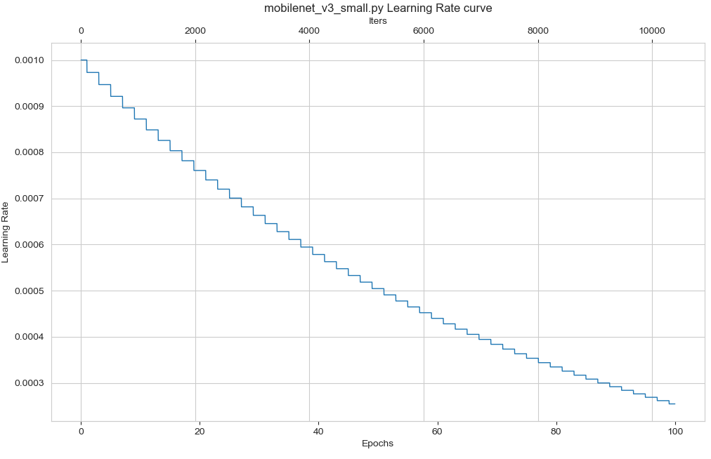
示例Step:
python tools/vis_lr.py models/mobilenet/mobilenet_v3_small.py
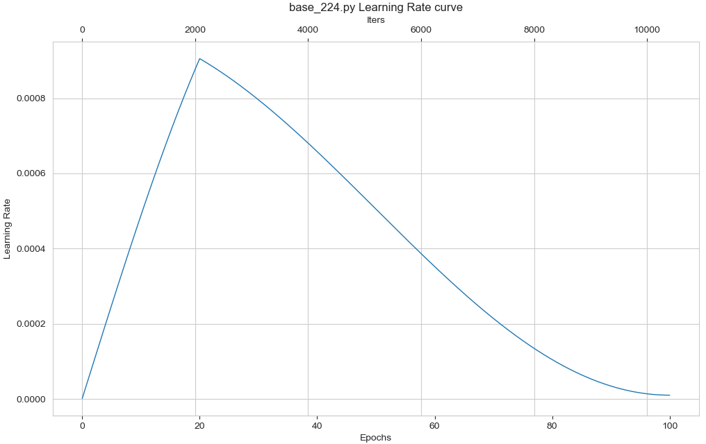
示例Cos:
python tools/vis_lr.py models/swin_transformer/base_224.py
预训练权重
名称权重名称权重名称权重
LeNet5
None
AlexNet
None
VGG VGG-11
VGG-13
VGG-16
VGG-19
VGG-11-BN
VGG-13-BN
VGG-16-BN
VGG-19-BN ResNet ResNet-18
ResNet-34
ResNet-50
ResNet-101
ResNet-152 ResNetV1C ResNetV1C-50
ResNetV1C-101
ResNetV1C-152 ResNetV1D ResNetV1D-50
ResNetV1D-101
ResNetV1D-152 ResNeXt ResNeXt-50
ResNeXt-101
ResNeXt-152 SEResNet SEResNet-50
SEResNet-101 SEResNeXt
None
RegNet RegNetX-400MF
RegNetX-800MF
RegNetX-1.6GF
RegNetX-3.2GF
RegNetX-4.0GF
RegNetX-6.4GF
RegNetX-8.0GF
RegNetX-12GF MobileNetV2 MobileNetV2 MobileNetV3 MobileNetV3-Small
MobileNetV3-Large ShuffleNetV1 ShuffleNetV1 ShuffleNetV2 ShuffleNetV2 EfficientNet EfficientNet-B0
EfficientNet-B1
EfficientNet-B2
EfficientNet-B3
EfficientNet-B4
EfficientNet-B5
EfficientNet-B6
EfficientNet-B7
EfficientNet-B8 RepVGG RepVGG-A0
RepVGG-A1
RepVGG-A2
RepVGG-B0
RepVGG-B1
RepVGG-A1
RepVGG-B1g2
RepVGG-B1g4
RepVGG-B2
RepVGG-B2g4
RepVGG-B2g4
RepVGG-B3
RepVGG-B3g4
RepVGG-D2se Res2Net Res2Net-50-14w-8s
Res2Net-50-26w-8s
Res2Net-101-26w-4s
ConvNeXt ConvNeXt-Tiny
ConvNeXt-Small
ConvNeXt-Base
ConvNeXt-Large
ConvNeXt-XLarge HRNet HRNet-W18
HRNet-W30
HRNet-W32
HRNet-W40
HRNet-W44
HRNet-W48
HRNet-W64 ConvMixer ConvMixer-768/32
ConvMixer-1024/20
ConvMixer-1536/20 CSPNet CSPDarkNet50
CSPResNet50
CSPResNeXt50 Swin Transformer tiny-224
small-224
base-224
large-224
base-384
large-384 Vision Transformer vit_base_p16_224
vit_base_p32_224
vit_large_p16_224
vit_base_p16_384
vit_base_p32_384
vit_large_p16_384 Transformer in Transformer TNT-small MLP Mixer base_p16
large_p16 Deit DeiT-tiny
DeiT-tiny distilled
DeiT-small
DeiT-small distilled
DeiT-base
DeiT-base distilled
DeiT-base 384px
DeiT-base distilled 384px Conformer Conformer-tiny-p16
Conformer-small-p32
Conformer-small-p16
Conformer-base-p16 T2T-ViT T2T-ViT_t-14
T2T-ViT_t-19
T2T-ViT_t-24 Twins PCPVT-small
PCPVT-base
PCPVT-large
SVT-small
SVT-base
SVT-large PoolFormer PoolFormer-S12
PoolFormer-S24
PoolFormer-S36
PoolFormer-M36
PoolFormer-M48 DenseNet DenseNet121
DenseNet161
DenseNet169
DenseNet201 Visual Attention Network(VAN) VAN-Tiny
VAN-Small
VAN-Base
VAN-Large Wide-ResNet WRN-50
WRN-101
Original: https://blog.csdn.net/zzh516451964zzh/article/details/125624528
Author: 啥都生
Title: 图像分类,看我就够啦!
原创文章受到原创版权保护。转载请注明出处:https://www.johngo689.com/661705/
转载文章受原作者版权保护。转载请注明原作者出处!